【代码】Financial Toolbox:Portfolio Optimization
对Matlab金融工具箱内的Portfolio_Optimization_Example代码的阅读笔记;
【Example】
打开文档
打开Matlab,在command中输入:
1 | |
可打开文档
加载数据
1 | |
初始化一个Portfolio对象
1 | |
AssetList:Asset名称的List,如果自己导入data,可采用:
1 | |
【可选步骤】
1.初始化一个 equal-weight portfolio
1 | |
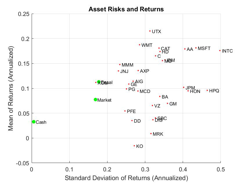
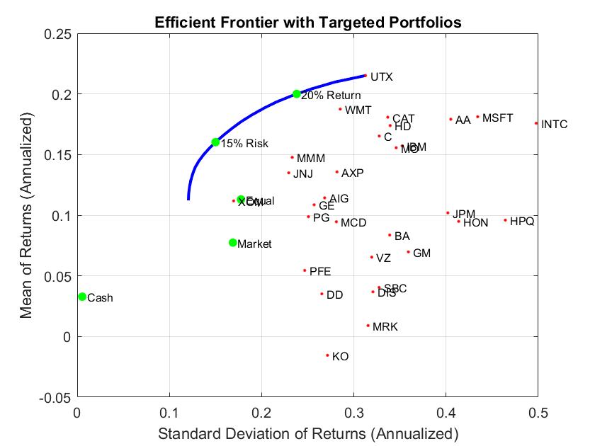
2.画一个所有Asset在risk-return上的分布图
1 | |
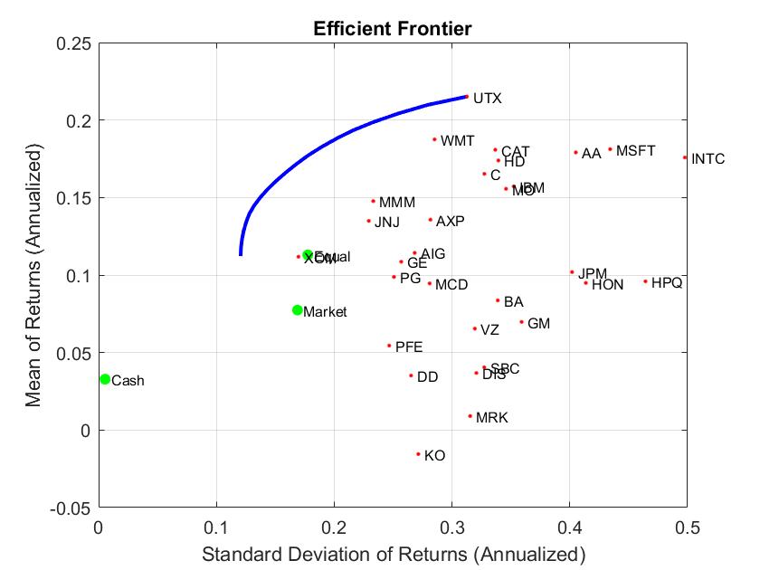
在各种约束下的投资组合优化
1.初始化一个long only portfolios
1 | |
2.初始化一个portfolios with budget constraint
1 | |
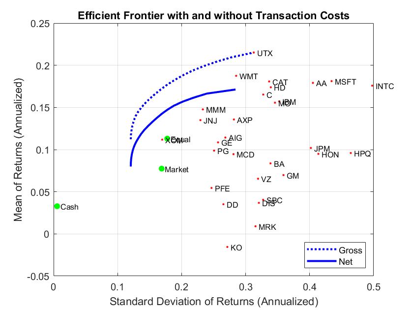
3.初始化一个portfolios其交易包含Transactions Costs
1 | |
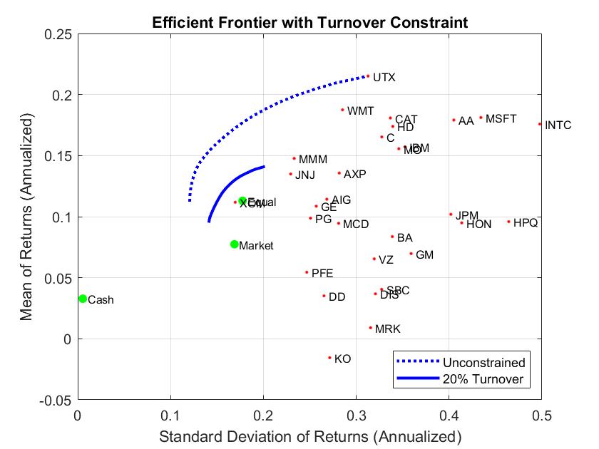
4.初始化一个portfolios其交易加入了Turnover Constraint
1 | |
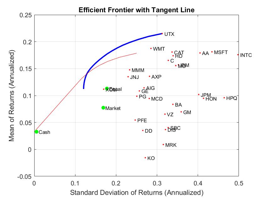
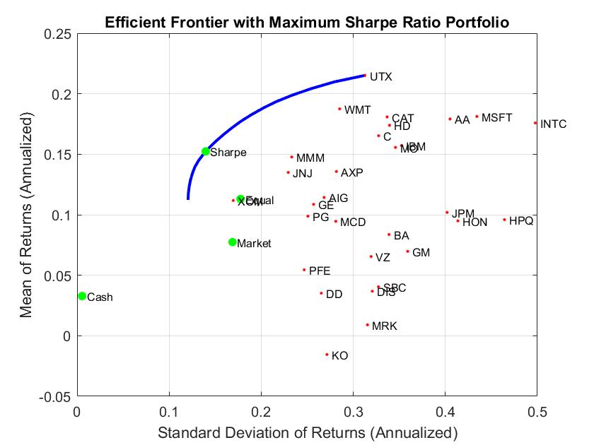
5.依照最大夏普比率得到最优组合
1 | |
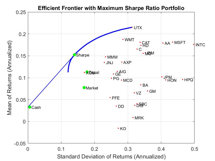
并与切线结合
1 | |
其他
1.获得risk和return的范围
1 | |
2.利用固定return或risk得到值
1 | |
3.显示portfolio的包含的Assets和weight占比
1 | |
Reference
【代码】Financial Toolbox:Portfolio Optimization
http://achlier.github.io/2021/03/11/Financial_Toolbox-Portfolio_Optimization/