【课程】金融科技工具箱
基于B站 up 无机言nokay 的视频《金融科技工具箱——面向经管金融同学的Python、爬虫、机器学习课》的笔记,此视频偏向面对金融系学生的基础讲解;
优点:快速入门,全面,有主讲人个人研究时的想法;
缺点:因为面向群众不是计算机系且时间有限,比较零碎,深入需要自学;
0. 其他资料
1. 基础部分
- 跳过,有时间另外整一版统一复习
1.5 数据结构
用于导出$Jason$的数据结构,爬虫时应该会用到
1 | |
导出/导入$Jason$文件
1 | |
1.6 常用函数
$cmd$操作
1 | |
按位
1 | |
复制
1 | |
打乱
1 | |
计个时
1 | |
查看文档
1 | |
1.7 作业
有趣的$tips$
1 | |
画红❤
1 | |

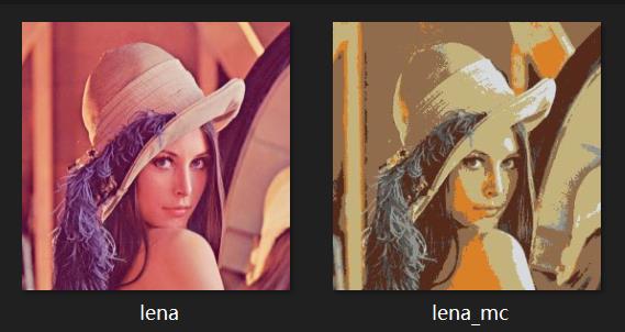
图片颜色代替(不提供材料,可在原视频下载)
1 | |
2. Numpy和Pandas
2.1 Numpy
- $array$所有元素都会变成同一个格式
- 注意 $dtype$ 格式,有时候(格式不对会导致计算错误,如非10进制的格式)
初始化函数
1 | |
属性
1 | |
索引
- 更换新数字时如果$type$不同将无法替换
- 但如果是字符串包数字,可以放
- $array$内截取的部分是$point$,如果改动截取的部分,原矩阵也会改变
1 | |
变形,拼接和分裂
1 | |
函数
1 | |
Numpy中可用的聚合函数
| 函数名称 | 描述 | 函数名称 | 描述 |
|---|---|---|---|
| np.sum | 计算元素的和 | np.argmin | 找出最小值的索引 |
| np.prod | 计算元素的积 | np.argmax | 找出最大值的索引 |
| np.mean | 计算元素的平均值 | np.median | 计算元素的中位数 |
| np.std | 计算元素的标准差 | np.percentile | 计算基于元素排序的统计值 |
| np.var | 计算元素的方差 | np.quantile | 计算基于元素排序的统计值 |
| np.min | 找出最小值 | np.any | 验证任何一个元素是否为真 |
| np.max | 找出最大值 | np.all | 验证所以元素是否为真 |
1 | |
2.2 Pandas
初始化
1 | |
定位
1 | |
合并
1 | |
Group
1 | |
Jason转DF
1 | |
保存、读取
1 | |
3. 可视化
- 跳过,有时间另外整一版统一复习
- 可视化不只是画图,而是为了更好地表达(如:南丁格尔玫瑰图)
- 画图工具包$pyecharts$
4. 爬虫
- 跳过,有时间另外整一版统一复习
BeautifulSoup
1 | |
selenium
1 | |
API
- 高德地图,$FutuQuant,Tushare,RiceQuant$等
5. 自然语言处理
- 有监督算法的描述-情绪判断,作者识别
- 无监督算法的描述-主题模型,词嵌入
独热编码(One-Hot)
主要是采用N位状态寄存器来对N个状态进行编码
1 | |
5.1 词袋模型(bag of words)
1 | |
TF-IDF(term frequency–inverse document frequency)
TF用以评估一字词对于一个文章的重要程度
- $n_{i,j}$ 词 $i$ 在 $j$ 中出现的次数
IDF用以评估一字词对于一个文章的不相关程度
- $D$ 文章总数
- $\{j:t_i\in d_j\}$ 包含词 $t_i$ 的文件数目
时间转换工具
用于时间排序
1 | |
英文文章预处理
1 | |
分词
1 | |
以防万一,先保存
1 | |
添加停用词
1 | |
去除低频词
1 | |
小容量储存
1 | |
转为语料格式
1 | |
TF-IDF 模型
1 | |
更多可查看 gensim官方网站
5.2 主题模型
Unigram
step 1
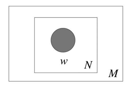
- $N:$ 文档
- $w:$ 词
- $Unigram$ 认为,每篇文章的词语是从一个独立多项式分布中抽取出来的
step 2
引入了一个主题的概念
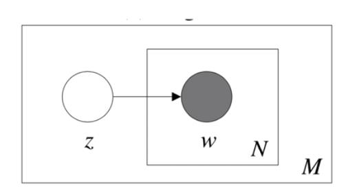
- $z:$ 主题
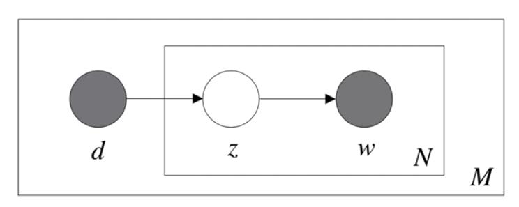
step 3
提出了混合主题,概率潜语义分析(pLSA/pLSI)
step 4
为参数引入先验分布,潜狄利克雷分布(LDA)
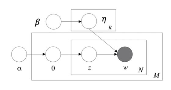
- 主题 $z$ 是一个参数为 $\theta$ 的多项式分布,这个参数的先验分布是一个参数为$\alpha$ 的狄利克雷分布
- 主题是否包含一个词是一个参数为 $\eta$ 的多项式分布,这个参数的先验分布是一个参数为 $\beta$ 的狄利克雷分布
- 如果主题数目为 $K$ ,则 $\alpha = 50/K$
- 如果词数量为 $W$ ,则 $\beta = 200/W $
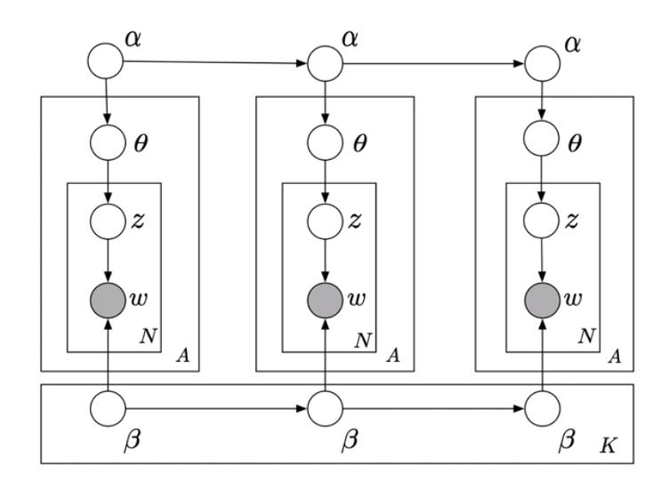
扩展
动态主题模型
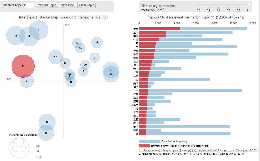
代码部分
1 | |
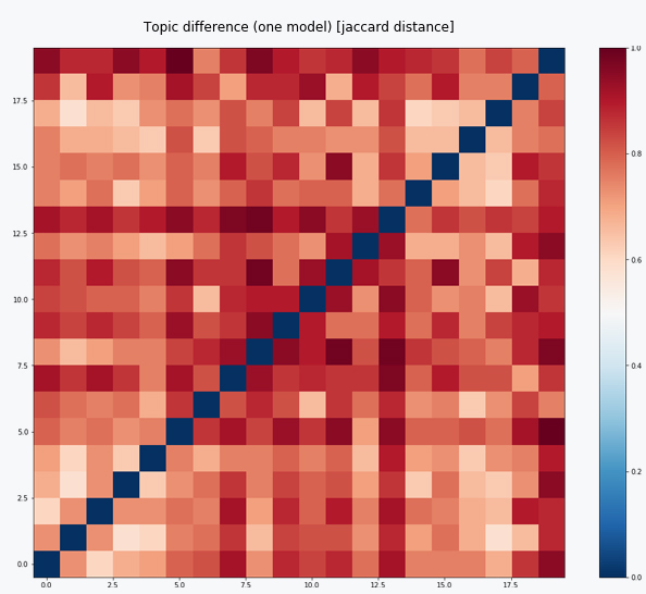
主题相关性检验
1 | |
1 | |
当集体颜色偏红,且对角一条为蓝点,则拟合成功
5.3 词向量模型
- $Word2vec$ 简单扩展:$doc2vec$
针对主题
1 | |
针对文章
1 | |
6. 机器学习
- 公式推导可参考B站另一视频【机器学习】【白板推导系列】【合集 1~23】
- 理论知识可阅读 林轩田机器学习基石 (本视频采用课件来源)+西瓜书+ESL
6.1 一些概念
监督学习
- 有监督 : 有标签的数据,人能指出的
- 无监督 : 无标签的数据,理论上无法给出完美答案
- 半监督 : 部分数据带标签, 如部分带标签的情绪识别
- 强化学习 : 含隐藏标签
训练过程
- $Batch$ 批处理 : 一次性训练所有数据
- $Online$ : 一批一批使用数据
- $Mini-batch$ : 以上两者结合
- $Active Learning$ : 机器自己选择需要的数据
数据类型
- 特征数据 : 有具体的含义
- 原始数据 : 图像声音本身
- 抽象数据 : 无意义的$UID$,主成分,其他中间结果
大数定律
由于不可能真正地存在完整的数据,输入数据$E_{in}(simple)$和真正完美的数据$E_{out}$ 必然存在误差;由于大数定理,及霍夫丁不等式 $(Hoeffding’s inequality)$ 得
如果$|E_{in}(h)-E_{out}(h)|$ 过大,则为坏数据
当存在$Breakpoint$, 则增长函数存在上限, 得$Vapnik-Chervonenkis (VC) bound$
因此,机器学习不仅要使$E_{in}$的误差尽量小,还需要使$E_{in}(h) \approx E_{out}(h)$ ;对此需要求得 $dvc (OLS,线性中为变量+1)$ , $N = 10 dvc$
6.2 线性回归
- $Lasso$ 和 岭回归 此类带正则的通常不是无偏, 而计量经济中多为对系数的解释,通常不用此方法
- 超参数($hyperparameter$)
6.3 SVM (Support Vector Machine)
$fewer dichotomies \to smaller ‘VC dim’$
$SVM$ 虽然不是无偏的,但 $B$ 变量可大于 $N$ 样本量
$CV(Cross-Validation)$ 交叉验证,可用 $K-Fold$ $(sklearn包)$
- 反向扩充(基础)
- $PLA(perceptron learning algorithm)$ -> $Pocket$算法 (前者改进)
- $KNN(k-NearestNeighbor)$
6.4 决策树 (Decision Tree)
节点选择/切分策略
- $ID3$算法,选择信息熵增大的最优算法
- $C4.5$算法,选择信息增益比最大的切分点,限制了$ID3$多切带来的过拟合
- $CART$算法,每一步切分使得数据正确率提升最多
停止切分
- 剩余数据$y$相同
- 剩余数据$x$相同
- 设定最小收益值
决策树的正则化
- 剪枝,减去几个带来收益最小的分叉节点
- $Early Stopping$,提升停止的最小值阈值
- 限制树高
实操建议
- 特征数量大容易过拟合
- 应预先进行维度压缩 $(PCA,ICA)$
- 对不同树的构建方法应有了解
- 提前将样本调平
- 把劣势数据复制多份
融合算法 (Blending)
- $t = 1,2,3…T$
- $D_t$ : the data at time $t$
- Obtain $g_t$ by $A(D)$
Bootstrap Aggregation (Bagging)
在$Size$为$N$的数据里面抽$N’$个数据作为第一个子样本,放回去,再抽$N’$个数据作为第二个子样本
随机森林 (Random Forest)
Out of Bag
- 当数据足够大时,一定有约等于 $\frac{1}{e}$的数据没有被抽取到
- 样本外数据可以用于 对$G$的$Validation$
- $G_N^-(x)=average(g_{没被用到的t})$
- $E_{oob}(G)=\frac{1}{N}\sum_{n=1}^Nerr(y_n,G_n^-(x_n))$
特征选择
- 变量重要性筛选 $permutation$ : 把变量打乱,$x_1 \to y_5$ ,差距越大越重要
- 对于$Dummy Variable$ 这种方法肯能会低估,因为打乱不充足
AdaBoost
- 计算$E_{in}$的时候,减少对做错过的$g_t$的$err$的权重
- 所有做错的权重只占1/2
- 当错$=n_1$,对$=n_2$
- $incorrect: u_n^{(t)}·n_2 \to u_n^{(t+1)}$
- $correct: u_n^{(t)}·n_1 \to u_n^{(t+1)}$
- $\epsilon_t = \frac{\sum_{n=1}^N u_n^{(t)}[y_n \neq g_t(x_n)]}{\sum_{n=1}^N u_n^{(t)}}$,$\Diamond_t=\sqrt\frac{1-\epsilon_t}{\epsilon_t}$,$\alpha_t=ln(\Diamond_t)$
- $incorrect: u_n^{(t)}·\Diamond_t \to u_n^{(t+1)}$
- $correct: u_n^{(t)}/\Diamond_t \to u_n^{(t+1)}$
- $G(x)=sign(\sum_{t=1}^T\alpha_tg_t(x))$
- 决策树中,在再抽样的步骤完成$u^{(t)}\to u^{(t+1)}$的变换(复制多份)
- 对于连续值:$GradientBoost$
6.5 编程的流程
- 数据的准备
- 数据的获取与存储方式
- 数据的标签化(特征化)
- 数据的清洗与预处理
- 方法的选择
- 合适的方法
- 合适的超参数
- 编程实现
- 工程流水线
- 标准流程
- 训练、测试集切分
- 正确的评价
- 结果呈现
- 表达准确
- 易于理解
- 飒
( 编程包 $sklearn$ )
7 深度学习
7.1 基础部分
- 对元和层的理解
- 单元数表达更细致的切分
- 多层表达更复杂的非线性组合方式
- $Sigmoid$
- 代替$sign$求导
- $S(x)=\frac{1}{1+e^{-x}}$
- $S’(x)=\frac{e^{-x}}{(1+e^{-x})^2}=S(x)(1-S(x))$
- $VC-dimension$
- $V = $神经元的数量, $D = $权重的数量 (前一个元数$+1$再乘后一个元数)
- 正则化
- $L2$正则, 由于$sign$中心趋近0,且为了保持可导,通常用其他方法
- $Early Stopping$
- 加入白噪音
- $Dropout$
- 发展进程
- $BP$神经网络(1986,$Hinton$)
- 手写体识别(1989,$LeCun$)
- 预处理 :权重训练方法的革新(2007,$Bengio$)
- 正式提出$CNN$(2012,$Hinton$)
- 图像分类,输入的是$3(RGB)\times224\times224$ (三维张量$tensor$)
7.2 卷积神经网络(CNN)
卷积
- $input$为一个矩阵
- 同时设定一个$filter$作为特征,和$step$值作为每次平移的步长
- $input$最左上角切割出一个同$filter$同大小的矩阵,并与其相乘,得到$output$中的第一块
- 按照步长平移最终得到完整的$output$
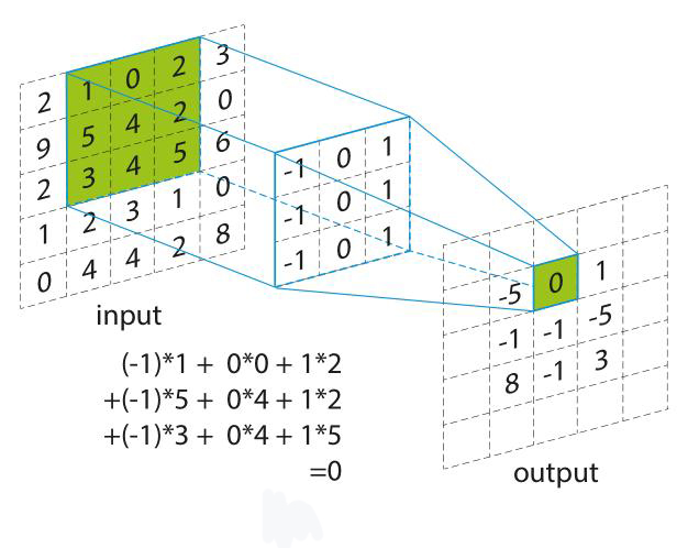
- 卷积神经网络中会取一个值$b$,$output=sign(output-b)$
- 达到了稀疏连接与参数共享的效果
Pooling
- 把数据变小,并保留最敏感的数$(Max Pooling)$
- 对应可放大缩小的性质
扩充
- 根据图片的特性推断,卷积神经网络适用于拥有以下特征的某些事物
- 小特征决定
- 放缩旋转存在
- 放大缩小不改变性质
- 不够数据的时候可以补0
7.3 循环神经网络(RNN)
- 把握时序特征($Recurrent NN$)
- 隐藏层有一个循环
- 历史输出端作为隐藏层的元素
- 双向$RNN$
- 当权重$w$跨过1的临界值时,如果迭代次数大,会有一个断崖式的变化,解决方法:
- $Clipping$
- $(2013,Pascanu)$
- $Long Short-Term Memory$
- $(1997,Sepp Hochreiter \& Jurgen Schmidhuber)$
- 建立遗忘门
- $Clipping$
7.4 聚类算法
算法总览
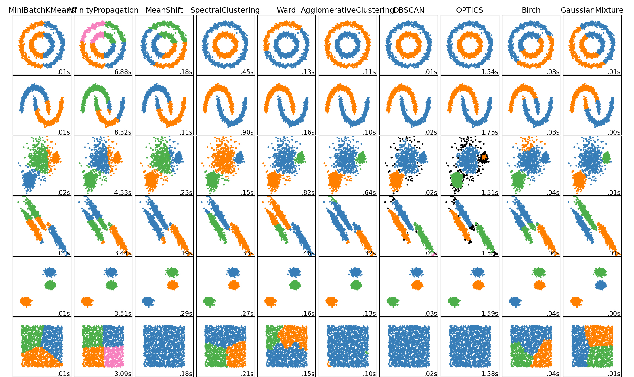
| Method name | Parameters | Scalability | Usecase | Geometry (metric used) |
|---|---|---|---|---|
| K-Means | number of clusters | Very large n_samples, medium n_clusters with MiniBatch code |
General-purpose, even cluster size, flat geometry, not too many clusters | Distances between points |
| Affinity propagation | damping, sample preference | Not scalable with n_samples | Many clusters, uneven cluster size, non-flat geometry | Graph distance (e.g. nearest-neighbor graph) |
| Mean-shift | bandwidth | Not scalable with n_samples |
Many clusters, uneven cluster size, non-flat geometry | Distances between points |
| Spectral clustering | number of clusters | Medium n_samples, small n_clusters |
Few clusters, even cluster size, non-flat geometry | Graph distance (e.g. nearest-neighbor graph) |
| Ward hierarchical clustering | number of clusters or distance threshold | Large n_samples and n_clusters |
Many clusters, possibly connectivity constraints | Distances between points |
| Agglomerative clustering | number of clusters or distance threshold, linkage type, distance | Large n_samples and n_clusters |
Many clusters, possibly connectivity constraints, non Euclidean distances | Any pairwise distance |
| DBSCAN | neighborhood size | Very large n_samples, medium n_clusters |
Non-flat geometry, uneven cluster sizes | Distances between nearest points |
| OPTICS | minimum cluster membership | Very large n_samples, large n_clusters |
Non-flat geometry, uneven cluster sizes, variable cluster density | Distances between points |
| Gaussian mixtures | many | Not scalable | Flat geometry, good for density estimation | Mahalanobis distances to centers |
| Birch | branching factor, threshold, optional global clusterer. | Large n_clusters and n_samples |
Large dataset, outlier removal, data reduction. | Euclidean distance between points |
7.5 PCA
将数据投射为波动最大的$n$维
优点
- 缓解维度灾难,提高可视度
- 降噪,提高模型稳定性
- 特征独立
- 可以对数据进行放缩(各向同性)
风险
- $PCA$的根据源于训练集,可能会过拟合
- 如果在训练数据进行了放缩,那么测试集要进行同参数的$mean-shift$和$variance$
- 不要先放缩再分割样本
Auto-Encoder
- 输入输出长度相等
- 扩展:$Denoising AutoEncoder$
7.6 生成模型
- $GAN Generative Adversarial Network$
- 人脸生成
- 图片上色
- 照片补充
- 根据文字生成图片
8 特征工程
从数据到变量
8.1 结构化与缺失值
缺失值处理
- 先思考缺失本身是不是就是一种信息
- 确保缺失是纯随机的
- 缺失是在哪个环境造成的
- 原始收集环节/采集环节/清洗环节
- 是否可以承担删变量带来的风险
- 主要变量与控制变量,应该补上
- 其他缺失如果超过阈值(一般为60%),应该删去
- 处理方法
- $Sklearn 6.4$ 专门用于缺失值处理
- 单变量填充(固定值,统计值)
- 多变量填充,近邻填充
- 先分割再填充
结构化
- 数据
- 分类信息:性别,学历
- 文本信息:$one-hot$
- $Encoding$
- $Ordinary encoder$
- 0,1,2;
- $one-hot encoder$
- 类似计量中的方法:$FixedEffect$
- 0,1 ; 0,1 ; 0,1 ;
- $Ordinary encoder$
- $Embedding$ : 嵌入
- $Doc2vec$:每一段(篇)文章一个向量
- $Glove$:考虑上下文窗口之外的其他文本
- $Elmo$:考虑不同文本在不同环境下的变义
- 图片嵌入
- $VAE(variation auto-encoder)$
8.2 改变分布
正则项和系数有关系,而系数又和数据有关系,所以要先做标准化
树方法的正则化不是来自于对系数的惩罚,可省略
前奏
清洗异常值
变形,删除极端值($winsor$)
标准化
(变量-均值)/标准差
测试集的标准化按训练集来
$preprocessing.StandardScaler()+scaler.transform()$
其他类似处理
- $MinMaxScaler$
- $MaxAbsScaler$
非线性变化:不惜一切变正态分布
方法
- $Box-Cox$
- $Yeo-Johnson$
- $Quantile transform$
可以 $Lognormal,Ohi-squared,Weibull$
不建议 $Gaussian,Uniform,Bimodal$,会损失信息
改进了线性模型的预测能力
- 看$R^2$和$MAE$
连续值变成分段值
增强稳健性:对异常值和非线性
试用于分类算法:信用风险模型,征信模型
$preprocessing.KBinsDiscretizer()$
8.3 变量选择
$sklearn.feature_selection$
为什么
- 方法制约
- 解释制约
- 预测制约
- 实践制约
单变量选择
单纯地从一个变量数据的分布进行筛选:$variation$大
- $VarianceThreshold$:$variance$大于某值的
- $SelectKBest$:筛选$K$个$variance$最高
- $SelectPercentile$:筛选高于某个阈值的
- 用于回归方法的分布:$f_regression,mutual_info_regression$
- 用于分类方法的分布:$chi2,f_classif,mutual_info_classif$
多变量选择
多次共线性的影响
- 方差膨胀系数($variance inflation factor$)
- $VIF_i = \frac{1}{1-R_i^2}$
- 当$VIF>10(or 5)$时,可以删去
- 当变量比较重要,删去与它相关的变量
算法选择
最稳健的方法
- $SelectFromModel$ 统一接口
- 后台算法
- $L1-based$
- $Support vector based$
- $Tree based$
8.4 实践:金融风控
- 方法基础:评分卡模型,逻辑回归
- 变量处理:离散化
- 变量筛选:单变量,多变量
- 重要方法:$WOE$与$IV$
- $WOE_i = ln(\frac{py_i}{pn_i}) = ln(\frac{y_i/y_T}{n_i/n_T}) = ln(\frac{y_i/n_i}{y_T/n_T})$
- $IV_i = (py_i-pn_i)*WOE_i$
- $i = 1$ 是男生
- $py_1 : $男生违约占比
- $pn_1 : $男生不违约占比
- $y_1 : $男生违约数量
- $n_1 : $男生不违约数量
- $y_T : $总体违约数量
- $n_T : $总体不违约数量
| IV范围 | 预测效果 | 英文描述 |
|---|---|---|
| <0.02 | 几乎没有 | Useless for prediction |
| 0.02~0.1 | 弱 | Weak predictor |
| 0.1~0.3 | 中等 | Medium predictor |
| 0.3~0.5 | 强 | Strong predictor |
| >0.5 | 难以置信 | Suspicious or too good to be true |
9 训练框架
9.1 度量指标:二分类问题
一个标准
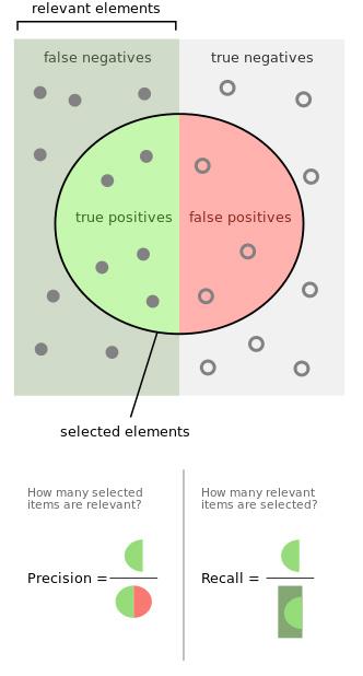
四个定义(数据-模型)
- $True-positives$:数据+,模型+
- $False-positives$:数据-,模型+
- $False-negatives$:数据+,模型-
- $True-negatives$:数据-,模型-
两个公式
- $Precision = True-positives$/ 模型+
- $Recall = True-positives$/ 数据+
一个指标:F1_score
另一个标准:ROC曲线与ROC面积(AUROC)
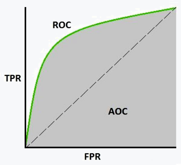
两个指标
- 真正例率($TPR$):召回的同义词 ,$sensitivity$
- $TPR = \frac{TP}{TP+FN}$
- 假正例率($FPR$)$specifity$
- $FPR = \frac{FP}{FP+TN}$
扩展:多分类问题
- 三个指标:F1_micro,F1_macro,F1_weighted
9.2 度量指标:回归
- $MAE = \frac{1}{N}\sum_{t=1}^N|y_i-\hat{y}|$
- $MSE = \frac{1}{N}\sum_{t=1}^N(y_i-\hat{y})^2$
- $RMSE = \sqrt{MSE}$
- $R^2 = 1-\frac{\sum(y_i-\hat{y})^2}{\sum(y_i-\bar{y})^2} = 1-\frac{MSE(\hat{y},y)}{Var(y)}$
9.3 超参搜寻
搜索方法
- $Grid Layout$
- $Random Layout$
- 步骤
- 阅读论文找范围
- 不同尺度的$Grid Layout$
- $Random Layout$
- 暴力手段之外
- $Model specific cross-validation$
- $AIC,BIC$
- $Out of Bag Estimates$
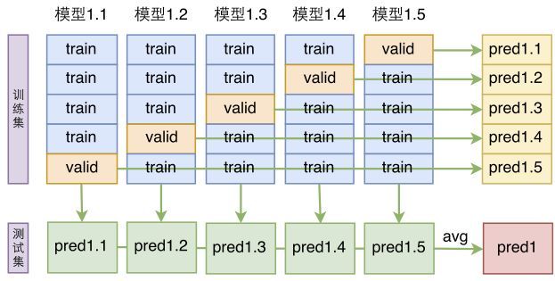
9.4 交叉验证
$sklearn.model_selection$
数据切割
训练数据(7)验证数据(2)测验数据(1)
时间上的泄漏:注意时序数据中途没有被其他情况影响
- 数据分组上的泄漏:一家人不能分开处理
- 统计特征上的泄漏:先分割后处理
怎么划分
- $KFold$
- 随机抽取 = $ShuffleSplit$
- 抽取时要保证类别间的平衡$= StratifiedShuffleSplit$
- 当有小组时 $= GroupKFold$
- 当有时间存在,训练集必须早于验证集 = $TimeSeriesSplit$
流程图
问题提出
文献搜集
- 做过吗
- 怎么做
- 与课题有何差别
- 能改什么方法
- 数据搜集
- 典型数据库
- 特异数据源
- 数据更新管理
- 成本控制
- 特征工程
- 抽取哪些变量
- 生成那些指标
- 是否要改特征
- 是否能改特征
- 模型选择
- 符合假设
- 能力优化
- 容易解释
- 开销合理
- 模型优化
- 变量
- 结构
- 超参数
- 训练技巧
- 结构呈现
- 数据可视化
- 关键词提炼
- 模型更新策略
- 边界与预警