【课程】Financial Markets Securities and Derivatives

基于格拉斯哥ECON5009的笔记；

General information

Aims

This course focuses on providing a broad overview of the financial markets with emphasis on pricing and hedging of different securities and derivatives. The issues related to trading of different financial instruments are discussed in detail and the option pricing methodology is taught using the basic market models such as the binomial model and Black-Scholes model. The course also teaches the construction of investment portfolios using interest rates-based instruments such as bonds and credit default swaps. The hedging techniques involving the computation of option Greeks are also covered. The practical implementation of many of the theoretical concepts is taught in the computer lab sessions using the Monte Carlo method.

ILOs

By the end of this course students will be able to:

1. Analyse the effectiveness of different models used in the financial markets
2. Calculate the price and hedging portfolios of popular derivatives traded in the financial markets
3. Formulate investment portfolios using interest-rates based financial instruments.

Unit 1: Mean Variance Analysis and the Capital Asset Pricing Model

Unit 1.1

Holding period return (including dividends) :

$$R_t = \frac{P_t-P_0+D_t}{P_0}$$

Discussion: why do we choose simple rate of return $\frac{Pt − P0}{P0}$ over log return $ln\frac{Pt}{P0}$ for portfolio analysis?

Because using the simple rate of returns implies that returns are additive

Unit 1.4

Variance of Portfolio

$$\sigma_p^2=w_1^2\sigma_1^2+w_2^2\sigma_2^2+2w_1w_2\sigma_{12}$$

Covariance

$$\begin{align} \sigma_{12}&=E((R_{1j}-E(R_1))(R_{2j}-E(R_2)))\\ &=E(R_1R_2)-E(R_1)E(R_2) \end{align}$$

The covariance measures the comovement of the returns on two assets.

Unit 1.5

Correlation Coefficient

$$\rho_{12}=\frac{\sigma_{12}}{\sigma_1\sigma_2}$$

The correlation coefficient measures the direction and strength of the comovement between two variables.

When ρXY = 1

$$\sigma_p = w_x\sigma_x+w_y\sigma_y$$

When ρXY = -1

$$\begin{align} \sigma_p &= |w_x\sigma_x-w_y\sigma_y|\\ \sigma_p &=0,\ when \ w_x = \frac{\sigma_y}{\sigma_x+\sigma_y} \end{align}$$

Unit 1.6

Minimum-risk Portfolio

$$w_x = \frac{\sigma_y^2-\sigma_x\sigma_y\rho_{xy}}{\sigma_x^2+\sigma_y^2-2\sigma_x\sigma_y\rho_{xy}}$$

Maximum Sharp-ratio（推导步骤）

$$w_x =\frac{(\bar{R}_x-rf)\sigma_y^2-(\bar{R}_y-rf)\rho_{xy}\sigma_x\sigma_y}{(\bar{R}_x-rf)\sigma_y^2+(\bar{R}_y-rf)\sigma_x-(\bar{R}_x-rf+\bar{R}_x-rf)\rho_{xy}\sigma_x\sigma_y}$$

Efficient Frontier

The efficient set consists of the portfolio possibilities curve of all portfolios that lie between the global minimum-risk portfolio and the maximum expected return portfolio. This set of portfolios is called the efficient frontier.

Unit 1.7

Effectiveness of Diversification for Large Portfolios (N）

$$\begin{align} \sigma_p^2 &= \frac{1}{N}\sum_{j=1}^N(\frac{\sigma_j^2}{N})+ \frac{N-1}{N}\sum_{j=1}^N\sum_{k=1,k\ne j}^N(\frac{\sigma_{jk}}{N(N-1)})\\ &= \frac{1}{N}\bar{\sigma}_j^2+\frac{N-1}{N}\bar{\sigma}_{jk} \end{align}$$

Can be divided into:

1. Diversifiable risk / Unsystematic risk

   $$lim_{N\to \infty}(\frac{1}{N}\bar{\sigma}_j^2)=0$$

2. Undiversifiable risk / Systematic risk

   $$lim_{N\to \infty}(\frac{N-1}{N}\bar{\sigma}_{jk})=\bar{\sigma}_{jk}$$

Unit 1.8

Problems of Short Sales

1. Unlimited losses: the loss of a short sale can theoretically be infinite because the stock price can theoretically rise to infinity.

2. Short squeeze: the price of a heavily shorted stock suddenly increases sharply, forcing the short sellers to close out their short position.

3. Not working in the long run: historically, over long period of time, stock prices have positive drift.
4. Costs associated with margin trading: the minimum maintenance requirement must be met. As stock price increases, the value of margin call might be too high to be fulfilled by the investor.

Initial margin requirements : the Federal Reserve Board requires all short sale accounts to have 150% of the value of the short sale at the time the sale is initiated.

Maintenance margin requirements : it is 100% of market value of short sale plus at least 25% of total market value of securities in the margin account.

Unit 1.9

Other Methods to Reduce Short Sales Risk

1. Stop buy order: when the increasing stock price reaches the execution price, the order is executed to limit the loss.

2. Portfolio of two assets: short selling the asset with low return and use the proceeds to purchase the asset with high return.

3. Out-of-the-money call option: if underlying stock price increases, the investor can exercise the option and buy the stock at the strike price.

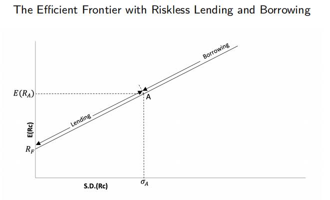
Unit 1.10

The Efficient Frontier with Riskless Lending and Borrowing

The expected return on the combination of riskless asset F and risky portfolio A is:

$$E(R_C)=w_FR_F+w_AE(R_A)$$

combinate with:

$$\begin{align} \sigma_C &= (w_F^2\sigma_{R_F}^2+w_A^2\sigma_A^2+2w_Aw_F\rho_{AF}\sigma_A\sigma_{R_F})^{\frac{1}{2}}\\ &= w_A\sigma_A \end{align}$$

Therefore, we have:

$$E(R_C)=R_F+(\frac{E(R_A)-R_F}{\sigma_A})\sigma_C$$

Unit 1.13

The Single-Index Model

$$R_i=a_i+\beta_iR_m$$

a is the component of security’s return that is independent of the return of the market index.

β is a constant that measures how sensitive a security’s return is to the return on the market index.

β > 1: stock is riskier than the market.

we assume that:

$$a_i = \alpha_i+e_i$$

Therefore, we have:

$$R_i=\alpha_i+\beta_iR_m+e_i$$

Variance of Single-Index Model

$$\sigma_p^2=\sum_{i=1}^Nw_i^2\beta_i^2\sigma_m^2+\sum_{i=1}^N\sum_{j=1,i\ne j}^Nw_iw_j\beta_i\beta_j\sigma_m^2+\sum_{i=1}^Nw_i^2\sigma_{ei}^2$$

With N Portfolios, This is a total of merely 3N + 2 estimates. By contrast, when analysing portfolio without the Single-Index Model, the total number of estimates is 2N + N(N − 1)/2.

Unit 1.14

Variance can be directly written as :

$$\sigma_p^2=\beta_p^2\sigma_m^2+\sum_{i=1}^Nw_i^2{\sigma_{ei}^2}$$

assuming $w_i = 1/N$

$$\sigma_p^2=\beta_p^2\sigma_m^2+\frac{1}{N}\bar{\sigma}_{ei}^2$$

Can be divided into:

1. Diversifiable risk / Unsystematic risk / nonmarket risk

   $$lim_{N\to \infty}(\frac{1}{N}\bar{\sigma}_{ei}^2)=0$$

2. Undiversifiable risk / Systematic risk / market risk

   $$\beta_p^2\sigma_m^2$$

Unit 1.16

Capital Asset Pricing Model (CAPM)

$$E(R_i)=R_F+\beta_i(E(R_M)-R_F)$$

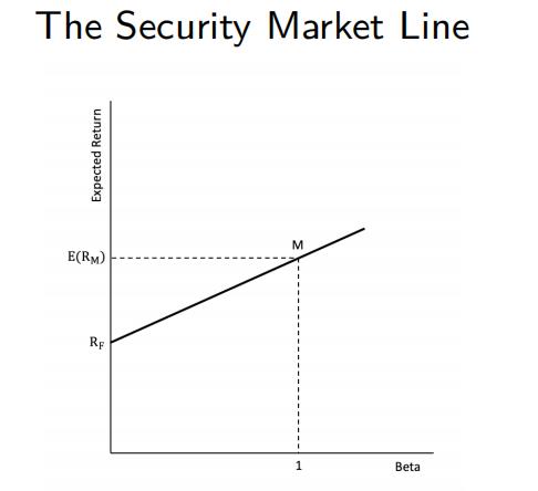
The higher the beta is for any security, the higher must be its equilibrium return.

This arbitrage would continue until all investments converged to the straight line. As a result, all investments and all portfolios of investments must lie along a straight line in expected return-beta space. This straight line is called the security market line.

Unit 1.21

From the results of the Single-Index Model:

$$\sigma_{iM} = \beta_i\beta_M\sigma_{M}^2 \to \beta_i = \frac{\sigma_{iM}}{\sigma_M^2}$$

replace the CAPM model:

$$E(R_i)=R_F+(\frac{E(R_M)-R_F}{\sigma_M})\frac{\sigma_{iM}}{\sigma_M}$$

we can also get that:

$$\sigma_i = \frac{\sigma_{iM}}{\sigma_M}$$

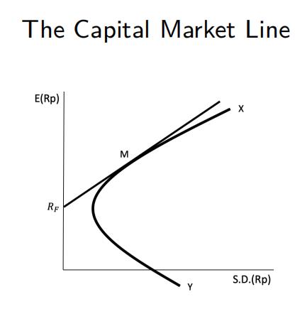
The straight line $R_F-M$ is referred to as the capital market line.

Where $\frac{E(R_M)-R_F}{\sigma_M}$ is referred to as the market price of risk for efficient portfolios.

$\frac{\sigma_{iM}}{\sigma_M}$ is the measure of how the risk on a security affects the risk of the market portfolio.

Unit 2: Forwards, Futures and Options

Unit 2.1

Forward Contracts

A forward contract is an agreement, i.e. a binding commitment, to buy or sell an asset at a certain future time for a certain price. A forward contract is traded in the over-the-counter market.

Futures Contracts

A futures contract is an agreement between two parties to buy or sell an asset at a certain time in the future for a certain price with (daily) clearing through a margin account. Unlike forward contracts, futures contracts are normally traded on an exchange. This suggests that, the exchange specifies certain standardized features of the contract

Margin Accounts

One of the key roles of the exchange is to use margin accounts to organize trading so that contract defaults are avoided. The extra funds deposited are known as a variation margin. If the investor does not provide the variation margin, the broker closes out the position by entering into the opposite trade to the original one.

Forward	Futures
traded in the OTC market	traded on the exchange
not standardized	standardized contract
usually one specified delivery date	range of delivery dates
settled at the expiry	settled daily
usually leading to delivery or cash settlement	usually closed out prior to maturity
some credit risk	virtually no credit risk

Unit 2.2

Continuous Compounding

$$lim_{m\to \infty}(1+\frac{R_m}{m})^{m}=e^{R_c}$$ $$R_c=m·ln(1+\frac{R_m}{m})$$

where $R_c$ denotes the annualized continuous-compounding yield; m is the compounding frequency; $R_m$ represents the annualized discrete-compounding yield.

Forward Price : $F_0=S_0e^{rT}$

Forward Price with coupon payment : $F_0=(S_0-G)e^{rT}$

Forward Price with Yield (continued) : $F_0=S_0e^{(r-q)T}$

The value of forward contract : $f_t=(F_t-K)e^{-(T-t)}$

Unit 2.4

Future price :

• if the interest rate rises, then the spot price is likely rising as well ⇒ due to the daily setllement in the futures contract, money can be released from the margin account and be invested at a higher interest rate
• if the interest rate falls, then the spot price is likely falling as well ⇒ due to the daily settlement, money needs to be paid into the margin account, but this money can now be borrowed at a lower interest rate
• relative to a forward contract, which is not affect by any of this, the futures contract benefits from interest rate movements, and this raises the futures price as compared to the forward price

Unit 2.6

Hedging

Short Hedges: a short hedge is a hedge that involves taking a short position in futures contracts.

• if the exposure is such that the company gains when the price of the asset increases and loses when the price of the asset decreases, a short hedge is appropriate.

Long Hedges: a long hedge is a hedge that involves taking a long position in futures contracts.

• if the exposure is such that the company gains when the price of the asset decreases and loses when the price of the asset increases, a long hedge is appropriate.

Cross Hedging: the asset underlying the futures contract is different from the asset whose price is being hedged.

• an airline may want to hedge the fluctuation in the price of jet fuel. Because futures on jet fuel are not actively traded, the airline could use heating oil futures contracts to hedge its exposure to jet fuel price fluctuation.

Hedge Ratio: the ratio of the size of the position taken in futures contracts relative to the size of the exposure.

• When cross hedging occurs, the hedger needs to choose a value for the hedge ratio such that the variance of the value of the hedged position is minimised. This value of the hedge ratio is referred to as the minimum variance hedge ratio.

Minimum Variance Hedge Ratio

Consider the case where the investor takes a long position in asset S and a

short position in the futures contract F.

• ∆S: change in spot price during a period of time equal to the life of the hedge;
• ∆F: change in futures price during a period of time equal to the life of the hedge;
• $σ_S$: standard deviation of ∆S;
• $σ_F$: standard deviation of ∆F;
• $ρ_{SF}$: correlation between ∆S and ∆F;
• h: minimum variance hedge ratio;
• ∆U = ∆S - h∆F: hedged position;

In order to find the min Var(∆U)

$$\begin{align} Var(∆U) &= Var(∆S - h∆F)\\ &= \sigma^2_S+h^2\sigma_F^2-2h\rho_{SF}\sigma_S\sigma_F \end{align}$$

$$\begin{align} \frac{\partial Var(∆U)}{\partial h} = 2h\sigma_F^2-2\rho_{SF}\sigma_S\sigma_F &= 0\\ \rho_{SF}\frac{\sigma_S}{\sigma_F} &= h \end{align}$$

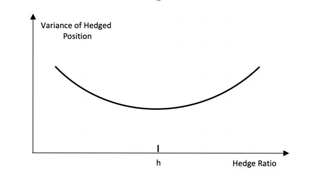
The hedge ratio is the slope coeffficient obtained from a linear regression of ∆S against ∆F.

Unit 2.7

Optimal Number of Contracts

• $N^*$: optimal number of futures contracts used for hedging;
• $Q_A$: size of position being hedged; e.g. number of units of assets
• $Q_F$: size of one futures contract; i.e the number of units of the underlying one future contract refers to

$$N^* = \frac{hQ_A}{Q_F}$$

Using Stock Index Futures to Hedge Equity Portfolios

• $V_A$: current value of the equity portfolio;
• $V_F$: current nominal value of one futures contract (i.e. the futures price times the contract size).
• each futures contract is on 250 times the index value.

If the portfolio mirrors the index : i.e. ρAF = 1 and σA = σF, the optimal hedge ratio h could be assumed to be 1.

$$N^* = \frac{V_A}{V_F}$$

In the case that the portfolio does not mirror the stock index

$$N^* = \beta \frac{V_A}{V_F}$$

Example

	T0	3 months
Value of S&P 500 Index	1000	900
S&P 500 futures price (short h)	1010	902
Value of the portfolio (long)	5050000	4286187
Risk-free interest rate	4% per annum	-
Dividend yield on index	1% per annum	-
Beta of the portfolio	1.5	-

$$N^* = 1.5 \times \frac{5050000}{250 \times 1010}=30$$

Gain form short:

$$30 \times (1010 - 902)\times 250 = 810000$$

Loss on stock index: $|(900-1000)/1000|=10\%$

Taking the dividends into accont: $-10\%+1\% \times 3/12 = -9.75\%$

The expected return on the portfolio can be computed as:$1\%+1.5\times(-9.75\%-1\%)=-15.125\%$

The expected value of the portfolio at the end of the 3 months: $5050000\times(1−15.125\%) = 4286187$

Thus, the expected value of the hedger’s position: $4286187 + 810000 = 5096187$

Unit 2.8

Option Contract

Option vs. Forward and Futures: it should be noted that an option gives the holder the right, but not the obligation, to buy or sell an asset.

Option Styles: depending on when the options can be exercised, options can be classified into European options and American options:

• European options: European options can be exercised only on the expiration date itself.

• American options: American options can be exercised at any time up to the expiration date.

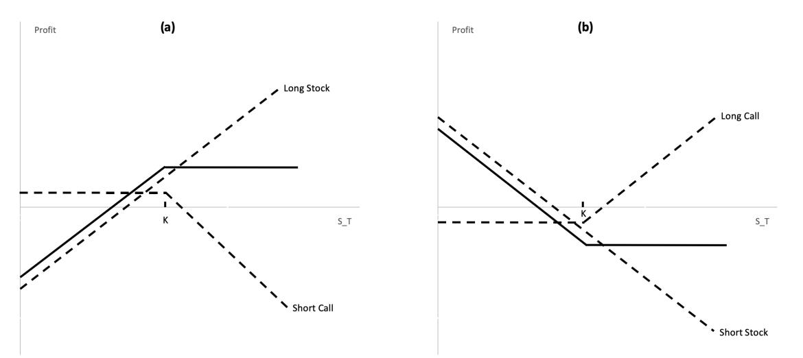
When the investor writes a call option, the investor’s position can either be covered or naked:

• Covered Call: a short position in a call option on an asset combined with a long position in the underlying asset.

• Naked Call: a short position in a call option that is not combined with a long position in the underlying asset.

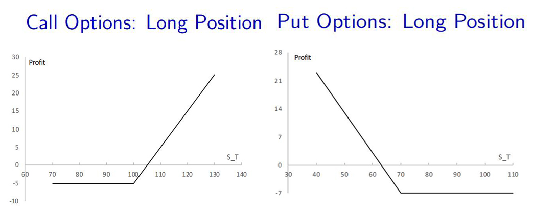
Intrinsic Value:

• intrinsic value of call option: $max(S_t − K, 0)$;

• intrinsic value of put option: $max(K − S_t, 0)$;

Moneyness:

• Call Option:

  • S > K: in the money
  • S = K: at the money
  • S < K: out of the money

• Put Option:

  • S < K: in the money
  • S = K: at the money
  • S > K: out of the money
• an option will be exercised only when it is in the money

Unit 2.9

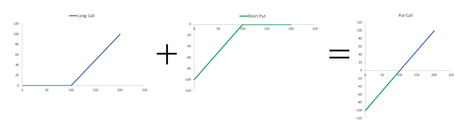
Put-Call Parity :

$$C + Ke^{−rT} = P + S_0$$ $$C − P = S_0 − Ke^{−rT} = (F_0 − K)e^{−rT} = f$$

Unit 2.10

Trading an Option and the Underlying Asset :

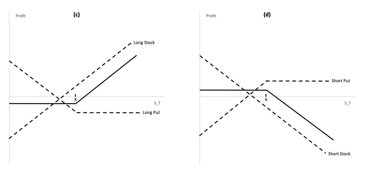
Bull Spread

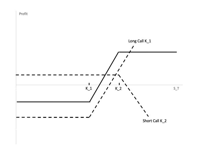
a bull spread limits both the upside profit potential and downside risk. The investor gives up some upside potential from the call with low K by selling another call with high K. In return for giving up the upside potential, the investor receives the up-front payment of the call with high K.

Bear Spread

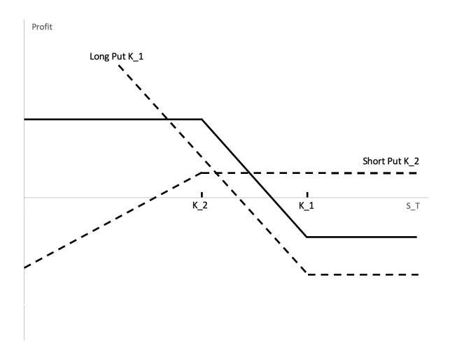
the bear spread limits both the upside profit potential and the downside risk. The investor gives up some of the upside profit potential by selling a put with a lower K. In return for the profit given up, the investor receives the up-front payment of the option sold.

Butterfly Spread

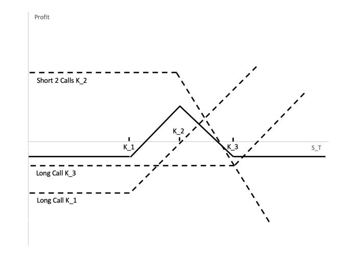
a butterfly spread leads to a profit if the stock price stays close to K2, but yields a small loss if there is a large stock price movement in either direction. Thus, a butterfly is appropriate when the investor expects that large stock price movement is unlikely

Straddle

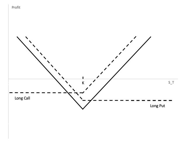
Strangle

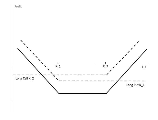
a straddle is usually purchased at the money by someone who expects the underlying asset to either rise or fall, but not to remain at the same level (i.e. bottom straddle or straddle purchase). For instance, a straddle could be bought just before the announcement of a company’s major news, on the announcement the company stock price could suddenly move either up or down.

Strangle & Strangle are volatility trades. Because of the relationship between the price of an option and the volatility of the asset, the investor can speculate on the direction of volatility.

Unit 3: Option Pricing: Binomial Model, Black Scholes Model, Volatility and Greeks

Unit 3.2

The option price derived from the risk-neutral valuation

In order to create a risk-free portfolio

$$\Delta = \frac{f_u-f_d}{S_0u-S_0d} , \ p = \frac{e^{rT}-d}{u-d}$$

The present value of the portfolio is

$$(S_0u\Delta-f_u)e^{-rT} \ or \ (pf_u+(1-p)f_d)e^{-rT}$$

The cost of setting up the portfolio is

$$S_0\Delta -f$$

Equation does not involve the real-world probability of stock pricesmoving up or down. Only the risk-neutral probability p is relevant in the binomial model.

Unit 3.5

Symmetric Random Walk ( process $M_k$)

$$X_j = \begin{cases}1 &\mbox{if }w_j = H, \\ -1 &\mbox{if }w_j = T,\end{cases}$$ $$M_0 = 0 \ , \ M_k = \sum_{j=1}^kX_j, \ k = 1,2,...$$ $$Var(M_{k_{i+1}}-M_{k_i}) = k_{i+1}-k_i$$

Brownian Motion W(t)

$$W^{(n)}(t) = \frac{1}{\sqrt{n}}M_{nt}\ ,\ W(t) \sim \epsilon \sqrt{t}\ , \ \epsilon \sim N(0,1)$$

Unit 3.6

Geometric Brownian motion (GBM)

A stochastic process $S_t$ is said to follow a geometric Brownian motion (GBM) if it satisfies the following stochastic differential equation (SDE):

$$dS_t = \mu S_tdt + \sigma S_tdW_t$$

Ito’s lemma for GBM:

$$dG = (\frac{\partial G}{\partial S}\mu S+\frac{\partial G}{\partial t}+\frac{1}{2}\frac{\partial^2 G}{\partial S^2}\sigma^2S^2)dt+\frac{\partial G}{\partial S}\sigma SdW$$

Let $G = lnS$, we have:

$$\frac{\partial G}{\partial S} = \frac{1}{S},\ \frac{\partial^2 G}{\partial S^2} = -\frac{1}{S^2},\ \frac{\partial G}{\partial t} = 0$$

we obtain:

$$dlnS_t = (\mu - \frac{\sigma^2}{2})dt + \sigma dW_t$$

Taking the exponential:

$$S_t = S_0exp((\mu - \frac{\sigma^2}{2})t+\sigma W_t)$$

The solution to the GBM implies that:

$$lnS_T \sim N(lnS_0 + (\mu - \frac{\sigma^2}{2})T, \sigma^2T)$$

or：

$$ln\frac{S_T}{S_0} \sim N((\mu - \frac{\sigma^2}{2})T, \sigma^2T)$$

Unit 3.7

Deriving the BSM Partial Differential Equation

Assuming $\delta$ is the number of shares needed to hedge one call option.

$$\delta \sigma S \Delta W = \frac{\partial f}{\partial S}\sigma S \Delta W$$

where $\delta = \frac{\partial f}{\partial S}$ is called the delta of the option.

Define $\Pi$ as the value of this portfolio, therefore:

$$\Pi = -f + \frac{\partial f}{\partial S}S$$

The change in the value of portfolio during time interval ∆t is given by:

$$\Delta\Pi = -\Delta f +\frac{\partial f}{\partial S}\Delta S$$

yields:

$$\begin{align} \Delta\Pi &= -(\frac{\partial f}{\partial S}\mu S+\frac{\partial f}{\partial t}+\frac{1}{2}\frac{\partial^2 f}{\partial S^2}\sigma^2S^2)\Delta t-\frac{\partial f}{\partial S}\sigma S\Delta W+\frac{\partial f}{\partial S}(\mu S\Delta t + \sigma S\Delta W)\\ &= (-\frac{\partial f}{\partial t}-\frac{1}{2}\frac{\partial^2 f}{\partial S^2}\sigma^2S^2)\Delta t \end{align}$$

In the absence of arbitrage opportunities, the risk-free portfolio must instantaneously earn the risk-free rate r. Otherwise, there would be arbitrage opportunities. Therefore, we have:

$$\Delta \Pi = r \Pi \Delta t$$

Substituting equations above, we obtain the BSM partial differential equation:

$$\frac{\partial f}{\partial t}+rS\frac{\partial f}{\partial S}+\frac{1}{2}\sigma^2S^2\frac{\partial^2 f}{\partial S^2} = rf$$

其他方法

BSM European Option Pricing Formula:

$$\begin{align} c &= S_tN(d_1)- e^{-r (T-t)}KN(d_2)\\ p &= e^{-r (T-t)}KN(-d_2)- S_tN(-d_1) \end{align}$$

With:

$$\begin{align} d_1&=\frac{1}{\sigma \sqrt{T-t}}(ln\frac{S_t}{K}+(r+\frac{1}{2}\sigma^2)(T-t))\\ d_2&=\frac{1}{\sigma \sqrt{T-t}}(ln\frac{S_t}{K}+(r-\frac{1}{2}\sigma^2)(T-t))\\ &=d1 - \sigma \sqrt{T-t} \end{align}$$

推导步骤

Matlab function

[Call,Put] = blsprice(Price,Strike,Rate,Time,Volatility)

Factors affecting option prices

	European Call	European Put	American Cal	American Put
$S_t$	+	-	+	-
$K$	-	+	-	+
$T-t$	+	+	+	+
$r$	+	-	+	-
$\sigma$	+	+	+	+

Volatility

• Historical volatility :The volatility of a stock price can be estimated empirically from historical data.
• Implied Volatility :Implied volatility is the volatility parameter implied from market option price using the Black-Scholes-Merton option pricing formula.

Matlab function

Volatility = blsimpv(St,K,r,T − t, c)

Volatility Smile : Volatility smile is the relationship between implied volatility and strike price for a particular maturity.

• volatility smile

  • 之所以被称为“波动率微笑”， 是指价外期权和价内期权（out of money和 in the money）的波动率高于在价期权（at the money）的波动率，使得波动率曲线呈现出中间低两边高的向上的半月形，也就是微笑的嘴形，叫波动率微笑。

• volatility skew

  • volatility曲线从左到右向下倾斜。这种情况在股票期权中最常见，因为股票的put option是一种保险，通常供不应求。而有时改变$\Delta t$也会造成从smile到skew的转变。

Option Greeks , read more about it

Unit 4: Bonds, interest rate swaps and credit derivatives

Unit 4.1

Part 1

Introduction to Bond

Definition: A bond is a debt instrument requiring the issuer (also called the debtor or borrower) to repay to the lender/investor the amount borrowed plus interest over a specified period of time.

Type of Issuer: There are three types of bond issuers:

1. The government and its agencies (Treasury bonds, UK gilts, German bunds)
2. Municipal governments (municipal bonds or munis)
3. Corporations (corporate bonds)

Term to Maturity: The term to maturity of a bond is the number of years over which the issuer has promised to meet the conditions of the obligation.

• Short-term bonds (bills): maturities are between 1 to 5 years;
• Intermediate-term bonds (notes): maturities are between 5 to 12 years;
• Long-term bonds (bonds): maturities are longer than 12 years;

Principal: the principal value (or simply principal) of a bond is the amount that the issuer agrees to repay the bondholder at the maturity date. Also referred to as the redemption value, maturity value, par value, or face value.

Coupon Rate: the coupon rate, also called the nominal rate, is the interest rate that the issuer agrees to pay each year.

Yield to maturity (YTM)

$$P = \sum_{t=1}^n\frac{C_t}{(1+y)^t}+\frac{M}{(1+y)^n}$$

Spot Rate: The n-year zero-coupon interest rate is sometimes also referred to as the n-year spot rate, the n-year zero rate. In other words, the spot rate is the yield to maturity on the zero-coupon bond.

Bootstrap Method: A procedure for calculating the zero-coupon yield curve from market data.

Part 2

Duration

Duration is a measure of a bond’s price sensitivity to yield changes.

Macaulay duration:

$$[\frac{1C}{1+y}+\frac{2C}{(1+y)^2}+...+\frac{nC}{(1+y)^n}+\frac{nM}{(1+y)^n}]\frac{1}{P}$$

Macaulay duration is a measure of how long on average the holder of the bond has to wait before receiving cash payments.

Modified duration:

$$-\frac{dP}{dy}\frac{1}{P} = \frac{1}{1+y}\times Macaulay \ duration$$

Modified duration can be interpreted as the approximate percentage change in bond price for a 1-percent change in yield.

当按月计算，会有些不同

Percentage Price Change

$$Modified \ duration\times dy = -\frac{dP}{P}$$

Convexity measure

$$convexity \ measure = \frac{d^2P}{dy^2}\frac{1}{P}$$

the second derivative of the price equation is:

$$\frac{d^2P}{dy^2} = \sum_{t=1}^n \frac{t(t+1)C}{(1+y)^{t+2}}+\frac{n(n+1)M}{(1+y)^{n+2}}$$

Duration matching / Portfolio immunization: the strategy makes a portfolio relatively insensitive to interest rates.

Unit 4.2

Part 1

Interest Rate Swap: an exchange of a fixed rate of interest on a certain notional principal for a floating rate of interest on the same notional principal. The most popular (plain vanilla) interest rate swap is one where LIBOR is exchanged for a fixed rate of interest

London Interbank Offered Rate (LIBOR) is the rate of interest at which a bank with an AA credit rating is able to borrow from other banks.

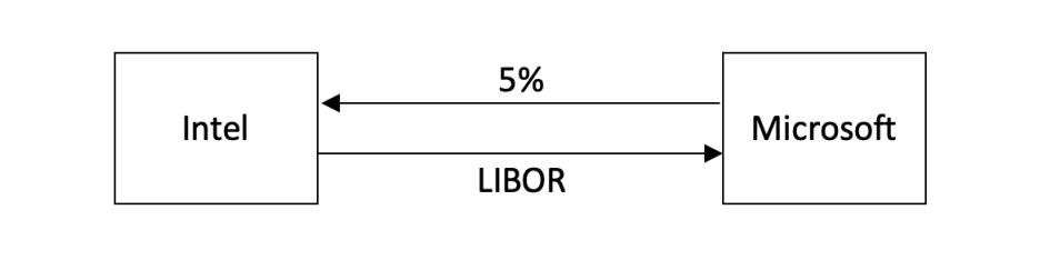
Example 1:

Microsoft agrees to pay Intel an interest rate of 5% per annum on a principal of 100 million, and in return Intel agrees to pay Microsoft the 6-month LIBOR rate on the same principal. In this case, Microsoft is the fixed-rate payer; Intel is the floating-rate payer.

Part 2

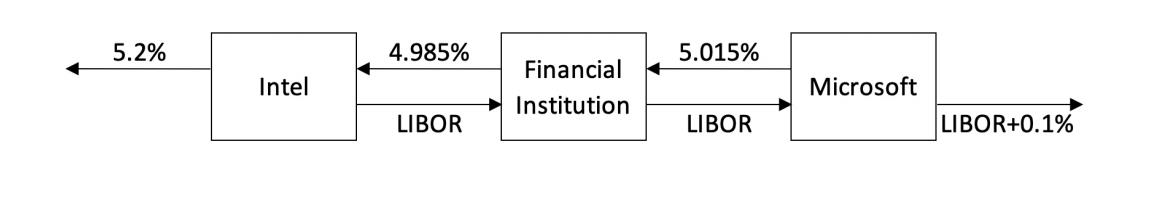
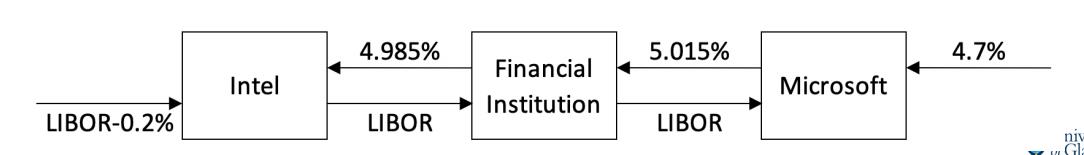
Role of Financial Intermediary: Usually two nonfinancial companies such as Intel and Microsoft do not get in touch directly to arrange a swap in the way indicated in Example 1. They each deal with a financial intermediary e.g. a bank or other financial institution. The LIBOR-for-fixed swaps are usually structured so that the financial institution earns about 3 or 4 basis points (0.03% or 0.04%) on a pair of offsetting transactions.

Example 2 Transform a Liability:

Microsoft has arranged to borrow 100 million at LIBOR plus 10 basis points (i.e. 0.1%). After Microsoft has entered into the swap, it has the following three cash flows:

• It pays LIBOR plus 0.1% to its outside lenders.

• It receives LIBOR under the terms of the swap.

• It pays 5.015% under the terms of the swap.

Suppose that Intel has a 3-year 100 million loan outstanding on which it pays 5.2%. After it has entered into the swap, it has the following three sets of cash flows:

• It pays 5.2% to its outside lenders.

• It pays LIBOR under the terms of the swap.

• It receives 4.985% under the terms of the swap.

Example 3 Transform an Asset:

Suppose that Microsoft owns 100 million in bonds that will provide interest at 4.7% per annum over the next 3 years. After Microsoft has entered into the swap, it has the following three cash flows:

• It receives 4.7% on the bonds.

• It receives LIBOR under the terms of the swap.

• It pays 5.015% under the terms of the swap.

Suppose that Intel has an investment of 100 million that yields LIBOR minus 20 basis points. After it has entered into the swap, it has the following three sets of cash flows:

• It receives LIBOR minus 20 basis points on its investment.

• It pays LIBOR under the terms of the swap.

• It receives 4.985% under the terms of the swap.

Part 3

Role of Market Makers: In practice, it is unlikely that two companies will contact a financial institution at the same time and want to take opposite positions in exactly the same swap. As a result, many large financial institutions act as market makers for swaps. This means that they are prepared to enter into a swap without having an offsetting swap with another counter-party. This type of swap is sometimes referred to as warehousing swap.

In general, the market makers quote, for different maturities, the bid and offer fixed rates they are prepared to exchange for the floating rate.

• Bid rate: the fixed rate that a swap market maker is prepared to pay in exchange for receiving LIBOR.

• Offer rate: the fixed rate that a swap market maker is prepared to receive in return for paying LIBOR.

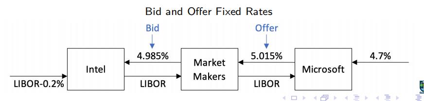
The average of the bid and offer fixed rates is known as the swap rate.

Credit risk refers to the risk that a loss will be experienced because of a default by the counterparty in a derivatives transaction.

The methods to reduce the credit risk include:

• Central Clearing: to reduce credit risk in over-the-counter swap markets, regulators require standardized over-the-counter derivatives to be cleared through central counterparties (CCPs). The CCP requires initial margin and variation margin from both sides in a transaction. LCH.Clearnet is the largest CCP for interest rate swaps.

• Credit Default Swaps (CDS): CDS is a swap that allows companies to hedge credit risks. A CDS is like an insurance contract that pays off if a particular company or country defaults.

Unit 4.3

Part 1

From the point of view of the floating-rate payer, a swap can be regarded as a long position in a fixed rate bond and a short position in a floating-rate bond, that is:

$$V_{swap} = B_{fix}-B_{fl}$$

From the point of view of the fixed-rate payer, a swap is a long position in a floating-rate bond and a short position in a fixed-rate bond, so that the value of the swap is:

$$V_{swap} = B_{fl}-B_{fix}$$

Valuation of Interest Rate Swaps in Terms of the Floating-rate Bond

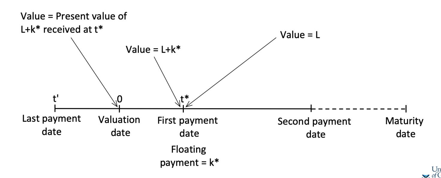
• $t’$: the last payment date

• $t^*$: first payment date (denoted by )

• except maturity: any other subsequent payment date
• $k^*$: the floating payment that be made at first payment date
• The floating-rate bond can therefore be regarded as an instrument providing a single cash flow of L + $k^*$ at first payment date.

Example 4:

Suppose that some time ago a financial institution agreed to receive 6-month LIBOR and pay 3% per annum (with semi-annual compounding) on a notional principal of 100 million. The swap has a remaining life of 1.25 years. The LIBOR rates with continuous compounding for 3-month, 9-month, and 15- month maturities are 2.8%, 3.2%, and 3.4%, respectively. The 6-month LIBOR rate at the last payment date was 2.9% (with semi-annual compounding).

Time	cc_rate	Bfix cash flow	Bfl cash flow	Discount factor	PV of Bfix cash flow	PV of Bfl cash flow
0.25	2.80%	1.5	101.45	0.993024443	1.489536664	100.7423297
0.75	3.20%	1.5		0.97628571	1.464428565
1.25	3.40%	101.5		0.958390466	97.27663225
				Sum	100.2305975	100.7423297
				V_swap	0.511732256

Part 2

Forward Rate

$$e^{R_F(T_2-T_1)}\times e^{R_1T_1} = e^{R_2T_2}\ ,\ or\ R_F = \frac{R_2T_2-R_1T_1}{T_2-T_1}$$

此处为连续的利率时计算，如果是非连续的

$$(1+R_1/n)^{T_1n}(1+R_F/n)=(1+R_2/n)^{T_2n}$$

Valuation of FRAs

$$V_{FRA}=L(R_K-R_F)(T_2-T_1)e^{-R_2T_2}$$

因为第一种得到的FRA是连续的，以上的是非连续的计算，所以有时需要进行转换，如果是连续的

$$V_{FRA}=L(e^{R_K(T_2-T_1)}-e^{R_F(T_2-T_1)})e^{-R_2T_2}$$

折现时的利率默认连续，如果不是需要进行转换

Part 3

Valuation of Interest Rate Swaps in Terms of FRAs

Example 5:

Under the terms of a swap, a financial institution has agreed to receive 6-month LIBOR and pay 3% per annum (with semiannual compounding) on a notional principal of 100 million. The swap has a remaining life of 1.25 years. The LIBOR rates with continuous compounding for 3-month, 9-month, and 15-month maturities are 2.8%, 3.2%, and 3.4%, respectively. The 6-month LIBOR rate at the last payment date was 2.9% (with semiannual compounding).

Time	cc_rate	RF_CC	RF_DD	fix cash flow	fl cash flow	Discount factor	PV of fix cash flow	PV of fl cash flow
0.25	2.80%	2.90%	2.90%	1.5	1.4500	0.993024443	1.489536664	1.439885442
0.75	3.20%	3.40%	3.43%	1.5	1.7145	0.97628571	1.464428565	1.673873318
1.25	3.40%	3.70%	3.73%	1.5	1.8672	0.958390466	1.437585698	1.789524424
						Sum	4.391550927	4.903283183
						V_swap	0.511732256

Unit 4.4

Part 1

Credit risk refers to the risk that a loss will be experienced because of a default by the counterparty in a derivatives transaction.

Credit derivatives allows companies to trade credit risk. These are contracts which involve cashflows/payoffs between two parties that are linked to the credit characteristics of another reference entity.

Types of Credit Derivatives

1. Event instruments: if a credit event, for example, a default can jeopardise your investment, then you may want to buy protection against that type of credit event by buying a credit default swap (CDS) providing a payoff that depends on the financial outcomes of that event.
2. Total return instruments: in this case you can transfer the financial gains of a credit risky asset against a pre-specified rate such as LIBOR plus a spread; examples are total return swaps.

The following definitions are useful in understanding of the functioning of CDS:

• Credit Event : a failure to make a payment as it becomes due, a restructuring of debt, or a bankruptcy.

• Reference Entity : a specified entity (sovereign, financial institution, corporation, or one among a basket of such specified entities).

• Protection Buyer : also the ‘Buyer’, the party paying a (periodic) fee in return for a contingent payment by the other party following a credit event of the reference entity.

• Protection Seller : also the ‘Seller’, the party receiving a (periodic) fee in return for making a contingent payment.

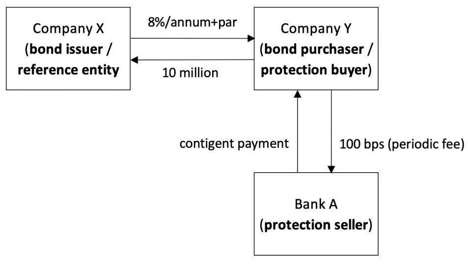
CDS Cash Flows

CDS generally includes three parties:

1. the issuer of the debt security (the reference entity)
2. the buyer of the debt security (protection buyer)
3. a third party who sells a CDS to the buyer of the debt security (protection seller)

CDS spread: The total amount paid per year, as a percentage of the notional principal, to buy protection.

Recovery Rate:

$$loss\ given\ default = 1 - recovery\ rate$$

The payoff from CDS is given as L(1 − R) where L is the notional principal and R is the recovery rate.

It then makes sense for the company to buy bonds on the reference entity such that the bonds are cheapest-to-deliver under the terms of CDS. That is, the bonds with minimum CDS-bond basis

$$CDS\_bond\_basis = CDS\_spead − Excess\_bond\_yield\_over\_risk-free\_rate$$

Part 2

Valuation of CDS

step 1: unconditional default and survival probabilities table

Suppose the default probability of the reference entity in the CDS is 2% in any year conditional on no earlier default.

Year	Default p	Survival p
1	0.02	0.98
2	0.0196	0.9604
3	0.019208	0.941192
4	0.01882384	0.92236816
5	0.018447363	0.903920797

step 2: Calculation of the Present Value of Expected Payments

Suppose that risk-free rate is 5% per annum with continuous compounding.

Suppose that a spread of s is paid per year to the protection seller on a notional principal of $1.

Year	Survival p	Expected payment	Discount factor	PV of payment
1	0.98	0.98	0.951229425	0.932204836
2	0.9604	0.9604	0.904837418	0.869005856
3	0.941192	0.941192	0.860707976	0.810091462
4	0.92236816	0.92236816	0.818730753	0.755171178
5	0.903920797	0.903920797	0.778800783	0.703974224
			Total	4.070447557

step 3: Calculation of the Present Value of Expected Accrual Payment

If a credit event occurs, it is assumed that it happens in the middle of the year. As the protection buyer makes the payment in arrears, we need to compute the expected accrual payment by protection buyer.

Year	Default p	Expected payment	Discount factor	PV of payment
0.5	0.02	0.01	0.975309912	0.009753099
1.5	0.0196	0.0098	0.927743486	0.009091886
2.5	0.019208	0.009604	0.882496903	0.0084755
3.5	0.01882384	0.00941192	0.839457021	0.007900902
4.5	0.018447363	0.009223682	0.798516219	0.007365259
			Total	0.042586647

step 4: Calculation of the Present Value of Expected Payoff

Suppose that the recovery rate is 40%.

Year	Default p	Expected payment	Discount factor	PV of payment
0.5	0.02	0.012	0.975309912	0.011703719
1.5	0.0196	0.01176	0.927743486	0.010910263
2.5	0.019208	0.0115248	0.882496903	0.0101706
3.5	0.01882384	0.011294304	0.839457021	0.009481083
4.5	0.018447363	0.011068418	0.798516219	0.008838311
			Total	0.051103977

The present value of the expected payments is the sum of total present value of the expected payments in the case of no credit event and total present value of the expected accrual payments in a credit event.

$$4.0704s+0.0426s=4.1130s$$

We choose the value of CDS spread s such that the present value of* expected CDS payments equals the present value of expected payoff from the CDS.

$$4.1130s = 0.0511$$

s = 0.0124. In other words, The mid-market CDS spread for the 5-year deal we have considered should be 0.0124 times the principal or 124 basis points per year.

Marking-to-market:

If CDS was entered at a spread value of 150 basis points.

$$4.1130 \times 0.0150 = 0.0617 > 0.0511$$

To the protection seller, the CDS would be worth $0.0617-0.0511 = 0.0106$ times the principal.

Other Types of CDS:

Binary CDS: It is a type of CDS which pays a fixed payoff of 1 dollar instead of 1 − R dollars in a credit event.

Basket CDS: In a basket CDS, there are more than one reference entity and a payoff is due when one or more reference entity defaults. There are different sub-types of a basket CDS

• Add-up basket CDS: provides a payoff when any one of the reference entities default.

• First-to-default CDS: provides a payoff only when the first default occurs.

• Second-to-default CDS: provides a payoff only when the second default occurs.

Part 3

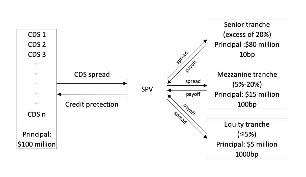
Collateralized Debt Obligation (CDO) is an asset-backed security which is backed by a diversified pool of assets such as investment grade and high-yield corporate bonds, residential mortgage-backed securities, bank loans, etc.

Typically, the payments and obligations based on the collected pool of CDSs are divided into different tranches: senior, mezzanine and junior or equity.

• senior: is considered almost without any risk. Receives the lowest CDS spread payments.

• equity: is based on the riskiest CDSs and is usually held by the originator itself or is sold to hedge funds.

• mezzanine: is based on the remaining CDSs and is the hardest tranche to sell.