【课程】Basic Econometrics

基于格拉斯哥ECON5002的笔记；

General information

This course introduces modern econometrics, focusing on regression analysis. The goal is to learn enough theory and get enough practice to be able to read journal articles and for conducting basic empirical research.

Aims

The aim of this course is to introduce modern econometrics. The goal is to learn enough theory and get enough practice to be able to read journal articles and for conducting basic empirical research. The emphasis is on applying econometrics to real-world problems. However, a solid understanding of the reviewed inference procedures will require rudiments of probability theory and statistics, and the ability to prove few basic results. The course focuses on regression analysis with cross-section data, under the familiar assumption of random sampling. This setting simplifies the exposition of the main results, requiring assumptions that are relatively straightforward yet realistic. The analysis of time series data is postponed to the last part of the course. This allows highlighting potential pitfalls that do not arise with cross-sectional data. Empirical exercises will be solved during computer lab sessions using an econometric software package.

ILOs

By the end of the course, students should be able to:

1. Derive some of the fundamental numerical and statistical properties of the OLS estimator.

2. Critically interpret a regression output to answer a given research question.

3. Critically evaluate the assumptions of the classical linear regression model and the ways they can be modified and with what effects.

4. Translate an economic argument into a formal testable hypothesis within a multiple regression model and implement the appropriate testing procedure.

5. Select the appropriate econometric tools and apply them to implement an empirical analysis using an econometric/statistical software package.

6. Communicate effectively, using appropriate technical terms.

7. Work collaboratively in a group to produce a combined output, by liaising with other class members, allocating tasks and co-ordinating

Unit 1：Introduction

Reading: Wooldridge, 7th Edition: Chapter 1

Definition:

Ceteris Paribus: Other factors being equal.

Quiz:

1. Income(x) has a causal effect on consumption(y).
2. A data set that consists of a variety of other units, taken at a given point in time, is called a(n) cross-sectional data set.

Unit 2：Regression Analysis: Estimation

Unit 2.1：The Simple Regression Model

Reading: Wooldridge, 7th Edition: Chapter 2, including Appendix 2A

Additional (Optional) Reading: Hansen (2020), Sections 2.1-2.9, 2.11, 2.14 and 2.15.

Definition:

Terminology for Simple Regression:

Y	X
Dependent variable	Independent variable
Explained variable	Explanatory variable
Response variable	Control variable
Predicted variable	Predictor variable
Regressand	Regressor

Simple Linear Regression Model:

$$y = \beta_0 + \beta_1x+u$$

• intercept parameter: $\beta_0$
• slope parameter: $\beta_1$

• error term: $u$

  population regression function (PRF):

  $$E(y|x)=\beta_0+\beta_1x$$

  The Ordinary Least Squares (OLS) Estimator:

  $$\begin{cases} \hat{\beta}_0 = \bar{y}-\hat{\beta}_1\bar{x}\\ \hat{\beta}_1 = \frac{\sum_{i=1}^n(x_i-\bar{x})(y_i-\bar{y})}{\sum_{i=1}^n(x_i-\bar{x})^2}=\frac{\hat{Cov}(x,y)}{\hat{Var}(x)} \end{cases}$$

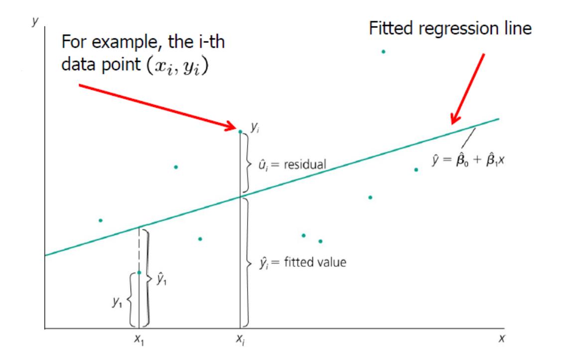
  OLS regression line/Sample Regression Function (SRF):

  $$\hat{y}_i = \hat{\beta}_0+\hat{\beta}_1x_i$$

  Residuals:

  $$\hat{u}_i = y_i - \hat{y}_i$$

  

Algebraic Properties of OLS statistics:

1. $\sum_{i=1}^n\hat{u}_i=0$
2. $\sum_{i=1}^n\hat{u}_ix_i=0$
3. $\bar{y}=\hat{\beta}_0+\hat{\beta}_1\bar{x}$
4. $\sum_{i=1}^n\hat{y}_i\hat{u}_i=0$
5. $\bar{y}=\frac{1}{n}\sum_{i=1}^n\hat{y}_i$

Measures of Variation:

• SST = $\sum_{i=1}^n(y_i-\bar{y})^2$
  • total sum of squares
• SSE = $\sum_{i=1}^n(\hat{y}_i-\bar{y})^2$=$\sum_{i=1}^n\hat{\beta}_1^2(x_i-\bar{x})^2$
  • explained sum of squares
• SSR = $\sum_{i=1}^n\hat{u}_i^2$
  • residual sum of squares
• SST = SSR+ SSR
• $R^2$ = $\frac{SSE}{SST}$ = $1-\frac{SSR}{SST}$, $0\leq R^2 \leq 1$
  • coefficient of determination

Summary of Functional Forms Involving Logarithms:

Model	Dependent Variable	Independent Variable	Interpretation of $\beta_1$
Level-level	y	x	$\Delta y=\beta_1\Delta x$
Level-log	y	log(x)	$\Delta y=(\beta_1/100)\%\Delta x$
Log-level	log(y)	x	$\%\Delta y=100\beta_1\Delta x$
Log-log	log(y)	log(x)	$\%\Delta y=\beta_1\%\Delta x$

Unbiasedness of OLS:

• Assumption SLR.1 (linearity in the parameters)

The random variables $(y_1,x_i)$ satisfy the linear regression equation

$$y_i=\beta_0+\beta_1x_i+u_i$$

• Assumption SLR.2 (random sampling)
• Assumption SLR.3 (sample variation in x)

$$0<Var(x_i)<\infty$$

• Assumption SLR.4 (Zero Conditional Mean)
  • $u_i uncorrelate with x$

$$E(u_i|x_i)=0$$

• Assumption SLR.2 and SLR.4 imply that the (Population) Regression Function is linear.
• Under Assumption SLR.1-SLR.4

$$E(\hat{\beta}_0)=\beta_0,\ and\ \ E(\hat{\beta}_1)=\beta_1$$

Variances of the OLS estimators:

• Assumption SLR.5 (homoskedasticity)

$$Var(u_i|x_i) = \sigma^2$$

• Under Assumptions SLR.1-SLR.5

$$Var(\hat{\beta}_1|x)=\frac{\sigma^2}{\sum_{i=1}^n(x_i-\bar{x})^2}=\frac{\sigma^2}{SST_x}$$ $$Var(\hat{\beta}_0|x)=\frac{\sigma^2n^{-1}\sum_{i=1}^nx_i^2}{\sum_{i=1}^n(x_i-\bar{x})^2}$$ $$E(\hat{\sigma}^2)=\sigma^2,\ \ \hat{\sigma}^2 = \frac{\sum_{i=1}^n \hat{u}_i^2}{n-2}$$

Not robust: The expectation is sensitive to perturbation in the tails of the distribution.

y on x

Quiz:

1. when the regression equation passes through the origin. $y_i=\beta_1x_i+u_i$
   • $\beta_1 = \frac{\sum_{i=1}^nx_iy_i}{\sum_{i=1}^nx_i^2}$
2. The observed values of $x$ span a wide range $\to$ SLR.3

Unit 2.1：The Multiple Regression Model

Reading: Wooldridge, 7th Edition: Chapter 3, including Appendix 3A. Chapter 6, Sections 6.1-6.3.

Additional Reading: Hansen (2020), Section 2.30

Definition:

Multiple Linear Regression Model:

$$y = \beta_0 + \beta_1x_1+\beta_2x_2+...+\beta_kx_k+u$$

• intercept parameter: $\beta_0$
• slope parameter: $\beta_1,…,\beta_k$

Unbiasedness of OLS:

• Assumption MLR.1 (Linear in Parameters)

• Assumption MLR.2 (Random Sampling)

• Assumption MLR.3 (No Perfect Collinearity)

In the sample (and in the population), none of the explanatory variables is constant, and there are no exact linear relationships among them.

• Assumption MLR.4 (Zero Conditional Mean)

$$E(u_i|x_{1i},x_{2i},...,x_{ki})=0$$

• Under Assumption MLR.1-MLR.4

$$E(\hat{\beta}_j)=\beta_j, \ \ for\ j = 0,1,...,k$$

Omitted Variable Bias:

We should have estimated

$$\hat{y} = \hat{\beta}_0+\hat{\beta}_1x_1+\hat{\beta}_2x_2$$

but we estimate

$$\tilde{y} = \tilde{\beta}_0+\tilde{\beta}_1x_1$$

Recall that

$$\hat{x}_2 = \tilde{\delta}_0+\tilde{\delta}_1x_1$$ $$\hat{y} = \hat{\beta}_0+\hat{\beta}_2\tilde{\delta}_0+(\hat{\beta}_1+\hat{\beta}_2\tilde{\delta}_1)x_1+\epsilon$$ $$\tilde{\beta}_1 =\hat{\beta}_1+\hat{\beta}_2\tilde{\delta}_1$$

Bias $(\tilde{\beta}_1|x)$=$\beta_2\tilde{\delta}_1$

if $ n \to \infty$, bias will approach $\frac{Cov(x_{1i},x_{2i})}{Var(x_{1i})}\beta_2$

	$Corr(x_1,x_2)>0$	$Corr(x_1,x_2)<0$
$\beta_2>0$	Positive bias	Negative bias
$\beta_2<0$	Negative bias	Positive bias

Variance of the OLS Estimators:

• Assumption MLR.5 (Homoskedasticity)

$$Var(u_i|x_{1i},x_{2i},...,x_{ki})=Var(u_i)=\sigma^2$$

• Assumptions MLR.1 through MLR.5 are called the Gauss Markov assumptions.

• Under Assumptions MLR.1 to MLR.5

  • $SST_j = \sum_{i=1}^n(x_{ij}-\bar{x}_j)^2$
  • $R_j^2$ is the $R^2$ of the regression

$$Var(\hat{\beta}_j|x)=\frac{\sigma^2}{SST_j(1-R_j^2)},\ \ j=1,2,...,k$$

• As $R_j^2 \to 1$, $Var(\hat{\beta}_j) \to \infty$ (the estimate of $\beta_j$ is not precise).
• Under the Gauss-Markov assumptions (MLR.1 through MLR.5)
  • standard deviation: $\sigma$; standard error: $\hat{\sigma}$
  • The square root of $\hat{\sigma}^2$,$\hat{\sigma}$, is reported by all regression packages (standard error of the regression, or RMSE).

$$\hat{\sigma}^2 = (n-k-1)^{-1}\sum_{i=1}^n\hat{u}_i^2 = SSR/df$$

• Under Assumptions MLR.1 through MLR.5
  • the OLS estimators are the best linear unbiased estimators (BLUEs)

Variances in Misspecified Models:

We run the misspecified and the correctly specified regressions

$$\begin{align} \tilde{y} &= \tilde{\beta}_0+\tilde{\beta}_1x_1\\ \hat{y} &= \hat{\beta}_0+\hat{\beta}_1x_1+\hat{\beta}_2x_2 \end{align}$$

Whenever $x_{1i}$ and $x_{2i}$ are correlated, $R_1^2 > 0$, and

$$Var(\tilde{\beta}_1|x)=\frac{\sigma^2}{SST_1}<\frac{\sigma^2}{SST_1(1-R_1^2)}<Var(\hat{\beta}_1|x)$$

• we can in fact get an estimator with a smaller variance, even though it is biased.

Adjusted R-Squared:

$$\bar{R}^2 = 1-\frac{[SSR/(n-k-1)]}{[SST/(n-1)]} = 1-\frac{\hat{\sigma}^2}{\hat{\sigma}_y^2}$$

Quiz:

1. Exclusion of a relevant variable from a multiple linear regression model leads to the problem of misspecification of the model.
2. An explanatory variable is said to be endogenous if it is correlated with the error term.

Unit 3：Regression Analysis: Inference

Definition:

Normal distribution in a nutshell

If $x\sim N(\mu,\sigma^2)$, then​

$$Z = \frac{X-\mu}{\sigma}\sim N(0,1)$$

• Assumption MLR.6 (Normality of error terms)

$$u_i \sim N(0,\sigma^2)\ \ u_i\ independent\ of\ x_{1i},x_{2i},...,x_{ik}$$

• Under assumptions MLR.1 – MLR.6: Classical Linear Regression Model (CLRM) assumptions
  • with estimated standard deviation

$$\frac{\hat{\beta}_j-\beta_j}{se(\hat{\beta}_j)} \sim t_{n-k-1}$$

Note: The t-distribution is close to the standard normal distribution if n-k-1 is large.

Null hypothesis:

$$H_0:\beta_j = 0\ \ against\ \ H_1:\beta_j>0$$ $$Reject\ if\ t_{\hat{\beta}_j}>c_a\ \ ,\ \ where\ Pr(t>c_a = \alpha)$$

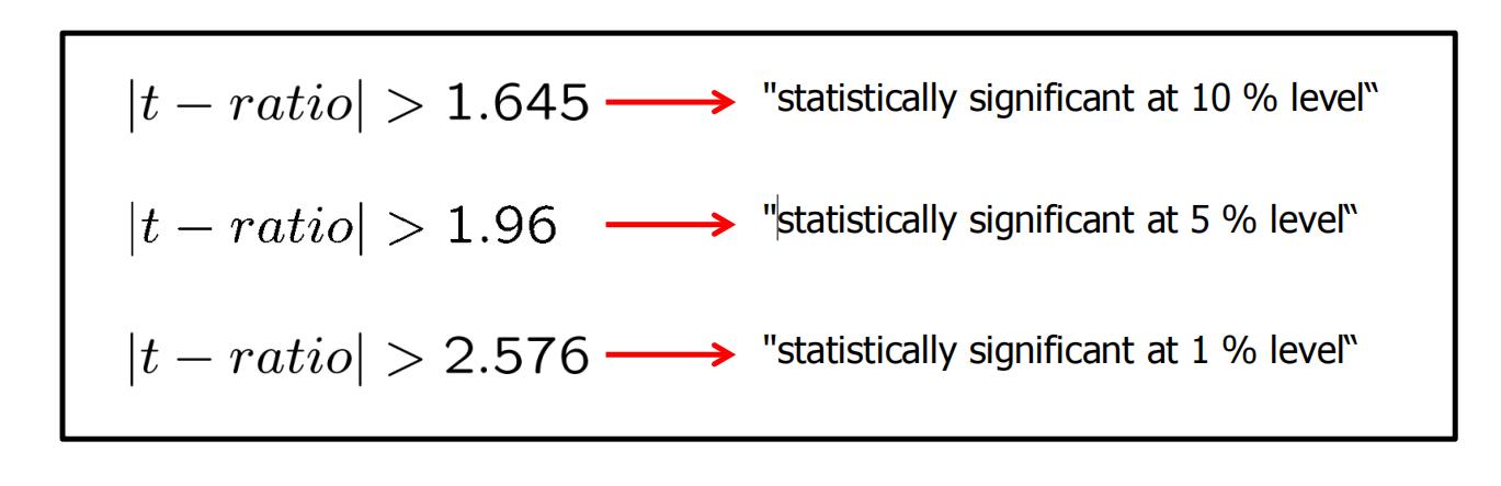
Statistically Significant:

Confidence Intervals:

The $\alpha\%$ confidence interval for $\beta_j$ is of the form

$$\hat{\beta_j}\pm c_a·se(\hat{\beta}_j) = 1-\alpha\ Confidence\ level$$

• $c_{0.01}=2.576,c_{0.05}=1.96,c_{0.10}=1.645$
• The effect is significantly different from zero if zero is outside the interval.
• It is not statistically significant if zero lies in the interval.

The difference between the estimates:

1. $t = \frac{\hat{\beta}_1-\hat{\beta}_2}{se(\hat{\beta}_1-\hat{\beta}_2)}$
2. Or Define $\theta_1 = \beta_1-\beta_2$ and test $H_0:\theta_1=0$

The F-test:

$$H_0:\beta_2=\beta_3=0$$ $$F = \frac{(SSR_r-SSR_{ur})/q}{SSR_{ur}/(n-k-1)}\sim F_{q,n-k-1}$$

$R^2$ form of the F –statistic:

$$SSR_r = (1-R^2_r)SST,\ \ \ SSR_{ur} = (1-R^2_{ur})SST$$ $$F = \frac{(R^2_{ur}-R^2_r)/q}{(1-R^2_{ur})/(n-k-1)}\sim F_{q,n-k-1}$$

Test of overall significance of a regression:

$$H_0:\beta_1=\beta_2=...=\beta_k=0$$ $$F = \frac{R^2/k}{(1-R^2)/(n-k-1)}\sim F_{k,n-k-1}$$

Testing general linear restrictions with the F-test:

$$H_0:\beta_1=1,\beta_2=...=\beta_k=0$$ $$x_i = y_i-x_{1i},\ \ SSR_r = \sum_{i=1}^n(x_i-\bar{x})^2$$

Quiz:

1. The significance level of a test is: the probability of rejecting the null hypothesis when it is true.
2. central limit theorem (CLT)
3. A restricted model will always have fewer parameters than its unrestricted model./ Degrees of freedom of a restricted model is always more than the degrees of freedom of an unrestricted model.
4. The ordinary least square estimators have the smallest variance among all the unbiased estimators.

Unit 4：Regression Analysis with Qualitative Information

Definition:

Dummy variable trap (perfect collinearity) :

When using dummy variables, one category always has to be omitted

Benchmark group

Chow test:

• $H_0$: equality of regression functions across two groups.

$$F = \frac{(SSR-(SSR_1+SSR_2)/k+1}{SSR_1+SSR_2/[n-2(k+1)]}$$

We can allow for an intercept difference between the groups, and then test for slope difference. Replace $SSR_p$ in Chow F-stat with the residuals from a regression with a dummy.

Quiz:

1. In a self-selection problem, the explanatory variables can be: endogenous.
2. Which of the following Gauss-Markov assumptions is violated by the linear probability model (LPM)?
   • The assumption of constant variance of the error term.
   • $Var(y|x)=p(x)[1-p(x)]$
3. Which of the following problems can arise in policy analysis and program evaluation using a multiple linear regression model?
   • The model can produce predicted probabilities that are less than zero and greater than one.
4. A problem that often arises in policy and program evaluation is that individuals (or firms or cities) choose whether or not to participate in certain behaviors or programs and their choice depends on several other factors. It is not possible to control for these factors while examining the effect of the programs.

Unit 5：Heteroskedasticity

Definition:

Heteroscedasticity: MLR.5 is violated.

Testing for heteroscedasticity:

Breusch-Pagan test:

$$\hat{u}^2 = \delta_0+\delta_1x_1+...+\delta_kx_k+error$$ $$H_0:\delta_1=\delta_2=...=\delta_k=0$$ $$F = \frac{R^2_{\hat{u}^2}/k}{(1-R^2_{\hat{u}^2})/(n-k-1)}\sim F_{k,n-k-1}$$ $$LM = n·R^2_{\hat{u}^2} \sim \chi_k^2$$

White test:

$$\begin{align} \hat{u}^2 &= \delta_0+\delta_1x_1+\delta_2x_2+\delta_3x_3\\ &+\delta_4x_1^2+\delta_5x_2^2+\delta_6x_3^2\\ &+\delta_7x_1x_2+\delta_8x_2x_3+\delta_9x_1x_3+error \end{align}$$ $$H_0:\delta_1=\delta_2=...=\delta_9=0$$ $$LM = n·R^2_{\hat{u}^2} \sim \chi_9^2$$

Alternative form of the White test:

$$\hat{u}^2 = \delta_0+\delta_1\hat{y}_1+\delta_2\hat{y}_2+error$$ $$H_0:\delta_1=\delta_2=0$$ $$LM = n·R^2_{\hat{u}^2} \sim \chi_2^2$$

Weighted least squares estimation:

$$Var(u_i|x_i)=\sigma^2h(x_i),h(x_i)=h_i>0$$

The functional form of the heteroscedasticity is known

set $w_i=\frac{1}{\sqrt{h_i}}$

$$\begin{align} y_i&=\beta_0+\beta_1x_{i1}+\beta_2x_{i2}+...+\beta_kx_{ik}+u_i\\ w_iy_i&=w_i\beta_0+w_i\beta_1x_{i1}+w_i\beta_2x_{i2}+...+w_i\beta_kx_{ik}+w_iu_i\\ y_i^* &=\beta_0x_{i0}^*+\beta_1x_{i1}^*+\beta_2x_{i2}^*+...+\beta_kx_{ik}^*+u_i^* \end{align}$$

where

$$E(u_i^{*2}|x_i)=\sigma^2$$

Observations with a large variance are less informative than observations with small variance and therefore should get less weight

Important special case of heteroscedasticity:

If the observations are reported as averages at the city/county/state/country/firm level, they should be weighted by the size of the unit. $\sigma^2/m_i$

Unknown heteroscedasticity function (feasible GLS) :

$$Var(u|x)=\sigma^2exp(\delta_0+\delta_1x_1+...+\delta_kx_k)=\sigma^2h(x)$$ $$\begin{align} u^2&=\sigma^2exp(\delta_0+\delta_1x_1+...+\delta_kx_k)·v\\ log(u^2)&=\alpha_0+\delta_1x_1+...+\delta_kx_k+e\\ \Rightarrow \hat{h}_i &= exp(\hat{\alpha}_0+\hat{\delta}_1x_1+...+\hat{\delta}_kx_k) \end{align}$$

White’s Heteroscedasticity-robust standard variance:

$$\hat{Var(\hat{\beta}_1)}_{HC}=\frac{\sum_{i=1}^n(x_1-\bar{x})\hat{u}_i^2}{[\sum_{i=1}^n(x_1-\bar{x})^2]^2}$$

Quiz:

1. A test for heteroskedasticty can be significant if
   • the functional form of the regression model is misspecified
   • Breusch-Pagan test/White test results in a small p-value
2. The generalized least square (GLS) is an efficient procedure that weights each squared residual by the:
   • inverse of the conditional variance of $u_i$ given $x_i$.
3. The heteroskedasticity-robust F statistic is also called the heteroskedastcity-robust Wald statistic.
4. The linear probability model contains heteroskedasticity unless all the slope parameters are zero.
5. The heteroskedasticity-robust t statistics are justified only if the sample size is large.
6. In weighted least squares estimation, less weight is given to observations with a higher error variance.
7. The WLS method fails if $\hat{h}_i$ is negative or zero for any observation.
8. The Hausman test is used to compare the Ordinary Least Squares (OLS) estimates and the Weighted Least Squares (WLS) estimates.
9. Multicollinearity among the independent variables in a linear regression model causes the heteroskedasticity-robust standard errors to be large.
10. The interpretation of goodness-of-fit ($R^2$) measures is unaffected by the presence of heteroskedasticty.

Unit 6：Regression Analysis with Time Series Data

Reading: Wooldridge 7th Edition Chapter 10: Basic Regression Analysis with the Time Series

Definition:

Finite distributed lag models:

In finite distributed lag models, the explanatory variables are allowed to influence the dependent variable with a time lag

Finite sample properties of OLS under classical assumptions:

• Assumption TS.1 (Linear in parameters)
• Assumption TS.2 (No perfect collinearity)
• Assumption TS.3 (Zero conditional mean)
  • (Contemporaneous) Exogeneity is not enough to ensure unbiasdness.

$$X = \begin{pmatrix}x_{11}&x_{12}&...&x_{1k}\\...&...&...&...\\ x_{t1}&x_{t2}&...&x_{tk}\\...&...&...&...\\ x_{n1}&x_{n2}&...&x_{nk}\\ \end{pmatrix}$$ $$\begin{align} Exogeneity&:\ E(u_t|x_t)=0\\ Strict\ exogeneity&:\ E(u_t|X)=0 \end{align}$$

• Unbiasedness of OLS

  • TS.1-TS.3 $\Rightarrow$ $E(\hat{\beta}_j)=\beta_j, j=0,1,…,k$

• Assumption TS.4 (Homoscedasticity)

  • $Var(u_t|X)=Var(u_t)=\sigma^2$

• Assumption TS.5 (No serial correlation)

  • $Corr(u_t,u_s|X)=0, t\neq s$
  • Three types of correlation:
    1. $Corr(x_{jt},x_{hs})$
    2. $Corr(x_{jt},xu{t})$
    3. $Corr(u_{t},u_{s})$

• OLS sampling variances

  • TS.1-TS.5 $\Rightarrow$ $Var(\hat{\beta}_j|X)=\frac{\sigma^2}{SST_j(1-R_j^2)}, j=0,1,…,k$$

• Unbiased estimation of the error variance

  • TS.1-TS.5 $\Rightarrow$ $E(\hat{\sigma}^2)=\sigma^2$

• Gauss-Markov Theorem:

  • Under assumptions TS.1 – TS.5, the OLS estimators have the minimal variance of all linear unbiased estimators of the regression coefficients

• Assumption TS.6 (Normality)

  • $u_t\sim iid N(0,\sigma^2)$ independent of $X$

• Normal sampling distributions

  • Under assumptions TS.1 – TS.6, the OLS estimators have the usual normal distribution (conditional on $X$ ). The usual F- and t-tests are valid.

Modelling a linear time trend:

$$y_t = \alpha_0+\alpha_1t+e_t$$

Modelling an exponential time trend:

$$log(y_t) = \alpha_0+\alpha_1t+e_t$$

Quiz:

1. a static model is postulated when a change in z at time t is believed to have an immediate effect on y
2. Adding a time trend can make an explanatory variable more significant if: the dependent and independent variables have different kinds of trends, but movement in the independent variable about its trend line causes movement in the dependent variable away from its trend line.
3. Time series regression is based on the assumption that no independent variable is constant nor a perfect linear combination of the others.
4. Which of the following assumption for time series analysis does not hold?
   • No serial correlation
5. One of the assumptions of time series regression is that there should be no serial correlation in the concerned series.
6. Cross-sectional regression rules out perfect collinearity among the regressors.
7. When a series has the same average growth rate from period to period, it can be approximated with an exponential trend.
8. Price indexes are necessary for turning a time series measured in nominal value into real value.

Unit 7：Further Issues Using OLS with Time Series Data

Reading: Wooldridge 7th Edition Chapter 11: Further Issues in Using OLS with Time Series Data

Definition:

Stationary stochastic processes:

A stochastic $\{x_t:t=1,2…\}$ process is stationary, if for every collection of indices $1\leq t_1\leq t_2\leq…\leq t_m$the joint distribution of $(x_{t_1},x_{t_2},…,x_{t_m})$ , is the same as that of $(x_{t_1+h},x_{t_2+h},…,x_{t_m+h})$ for all integers $h\ge1$.

Covariance stationary processes:

A stochastic process $\{x_t:t=1,2…\}$ is covariance stationary, if its expected value, its variance, and its covariances are constant over time:

1. $E(x_t)=\mu$
2. $Var(x_t)=\sigma^2$
3. $Cov(x_t,x_{t+h})=f(h)$

asymptotically uncorrelated：

when $h \to \infty, cov(x_t,x_{t+h}) \to 0$

Weakly dependent time series：

A stochastic process $\{x_t:t=1,2…\}$ is weakly dependent , if $x_t$ is “almost independent” of $x_{t+h}$ if $h$ grows to infinity (for all $t$).

Moving average process of order one (MA(1)):

$$x_t=e_t+\alpha_1e_{t-1}$$

Autoregressive process of order one (AR(1)):

$$y_t=\rho_1y_{t-1}+e_t \Rightarrow Corr(y_t,y_{t+h})=\rho_1^h$$

Asymptotic properties of OLS:

• Assumption TS.1‘ (Linear in parameters)
  • now the dependent and independent variables are assumed to be stationary and weakly dependent
  • Trend-stationary processes also satisfy assumption TS.1‘
• Assumption TS.2‘ (No perfect collinearity)

• Assumption TS.3‘ (Zero conditional mean)

  • Now the explanatory variables are assumed to be only contemporaneously exogenous rather than strictly exogenous

• Consistency of OLS：

  • TS.1‘-TS.3’ $\Rightarrow$ $plim\hat{\beta}_j=\beta_j, j=0,1,…,k$

• Assumption TS.4‘ (Homoscedasticity)

  • $Var(u_t|x_t)=Var(u_t)=\sigma^2$

• Assumption TS.5‘ (No serial correlation)

  • $Corr(u_t,u_s|x_t,x_s)=0, t\neq s$

• Asymptotic normality of OLS:

  • Under assumptions TS.1‘ – TS.5‘, the OLS estimators are asymptotically normally distributed. Further, the usual OLS standard errors, t-statistics and F-statistics are asymptotically valid

Random walks

$$y_t = y_{t-1}+e_t$$

• $E(y_t)=E(y_0)$
• $Var(y_t)=\sigma_e^2t$
• $Corr(y,y_{t+h}) = \sqrt{t/(t+h)}$

I(1) processes:

$$y_t=y_{t-1}+e_t \Rightarrow \Delta y_t=y_t-y_{t-1}=e_t$$

Testing for serial correlation

Testing for AR(1) with strictly exog. regressors :

$$H_0:\rho=0\ in\ \hat{u}_t=\rho\hat{u}_{t-1}+error$$

Durbin-Watson test under classical assumptions:

$$DW = \sum_{t=2}^n(\hat{u}_t-\hat{u}_{t-1})^2/\sum_{t=2}^n\hat{u}_t^2 \approx 2(1-\hat{\rho})$$

• $H_0 : \rho = 0$
• Reject if $DW d_U$, else the test is inconclusive.

When strictly exogeneity does not hold, t-test and DW test are not valid

Testing for AR(1) with general regressors:

$$\hat{u}_t=\alpha_0+\alpha_1x_{t1}+...+\alpha_kx_{tk}+\rho\hat{u}_{t-1}+error$$

• $H_0:\rho = 0$

General Breusch-Godfrey test for AR(q):

$$\hat{u}_t=\alpha_0+\alpha_1x_{t1}+...+\alpha_kx_{tk}+\rho\hat{u}_{t-1}+...+\rho_q\hat{u}_{t-q}+...$$

• $H_0:\rho_1=…=\rho_k = 0$

Correcting for serial correlation

with strictly exog. regressors:

$$\begin{align} y_t &= \beta_0+\beta_1x_t+u_t\\ \rho y_{t-1} &= \rho\beta_0+\rho\beta_1x_{t-1}+\rho u_{t-1}\\ \Rightarrow y_t-\rho y_t &= \beta_0(1-\rho)+\beta_1(x_t-\rho x_{t-1})+u_t-\rho u_{t-1} \end{align}$$ $$u_t=\rho u_{t-1}+e_t \Rightarrow u_t-\rho u_{t-1}=e_t$$

Newey-West formula:

• $\hat{\alpha}_t=\hat{r}_t\hat{u}_t$

$$\hat{v}=\sum_{t=1}^n\hat{a}_t^2+2\sum_{h=1}^g[1-h/(g+1)](\sum_{t=h+1}^n\hat{a}_t\hat{a}_{t-h})$$

• The integer g controls how much serial correlation is allowed:

  • g=2: $\hat{v}=\sum_{t=1}^n\hat{a}_t^2+\sum_{t=2}^n\hat{a}_t\hat{a}_{t-1}$
  • g=3: $\hat{v}=\sum_{t=1}^n\hat{a}_t^2+(4/3)\sum_{t=2}^n\hat{a}_t\hat{a}_{t-1}+(2/3)\sum_{t=3}^n\hat{a}_t\hat{a}_{t-2}$

• Serial correlation-robust standard errors:

  • $se(\hat{\beta}_j)=[“se(\hat{\beta}_j)/\hat{\sigma}”]^2\sqrt{\hat{v}}$

Quiz:

1. Which of the following is a strong assumption for static and finite distributed lag models?
   • Dynamic completeness
   • $E(y_t|x_t,y_{t-1},x_{t-1},…)=E(y_t|x_t)$
   • The problem of serial correlation does not exist in dynamically complete models.
2. sequentially exogenous
   • $E(u_t|x_t,x_{t-1},…)=E(u_t)=0$
3. A model with a lagged dependent variable cannot satisfy the strict exogeneity assumption.
4. A random walk process is not stationary.
5. Covariance stationarity focuses only on the first two moments of a stochastic process.
6. Under adaptive expectations, the expected current value of a variable adapts to a recently observed value of the variable.
7. A smaller standard error means: a larger t statistic.
8. Consistency of FGLS requires $u_t$ to be uncorrelated with $x_{t-1}$,$x_t$, and$x_{t+1}$
9. Prais-Winsten estimation is an example of FGLS estimation.
   • Prais-Winsten standard errors account for serial correlation, whereas OLS estimations do not.
10. Breusch-Godfrey test can be used to check for second order serial correlation.
11. The SC-robust standard errors work better after quasi-differencing a time series that is expected to be serially correlated.
12. Consistency of feasible generalized least square estimators requires the error term to be uncorrelated with lags of the explanatory variable. Correlation will lead to inconsistent estimates.
13. The Cochrane-Orcutt and Prais-Winsten methods are iterative methods of feasible generalized least square (FGLS) estimation.
14. The serial correlation-robust standard errors are typically larger than the usual OLS standard errors when there is serial correlation.