【课程】Economic Fundamentals and Financial Markets
基于格拉斯哥ECON5005的笔记;
General information
The aim of this course is to outline how macroeconomics fundamentals influence asset returns and asset prices.
Aims
The main aim of this course is to outline how macroeconomics fundamentals influence asset returns and asset prices.
ILOs
By the end of this course, students will be able to:
- Identify the role the financial sector plays in the economy at large, both in terms of resource allocation under uncertainty, trading of risk, and capital accumulation;
- Understand the determination of interest rates (using IS-LM and OLG);
- Identify the fundamental prices of basic financial assets, such as shares of stock, using state-of-the art techniques such as q-theory, real asset theory and monopolistic economic profit theory;
- Understand stock market price indices based on the market fundamentals implied by the previously mentioned theories.
Topic 1 – Macroeconomics and Financial Markets: The Gold Standard
Unit 1.1:Money, Paper Money and the Gold Standard
What is money?
- It is a means of payment
- It is a unit of account
- It is a store of value
Commodity and Fiat Money
- Commodity money are things with intrinsic value (gold, silver).
- Today’s paper money is called fiat money, because its value comes from government decree, or fiat.
Unit 1.2:Some History on the Gold Standard
A Brief History of Paper Money: The Role of Central Banking Link
A Brief History of Paper Money: The Role of the Gold Standard Link
Unit 1.3:Practical Implications of a Gold Standard Today
Dollar-gold exchange rate
- 55.12 dollar = 1 gram of gold
- $1 dollar=\frac{1 gram of gold}{55.12}=0.0181 grams of gold$
What would happen if the US tries to revert to this gold standard?
- Buffer stock problem
After simulated daily net inflows of cash and gold at the Fed during a year and cumulative net inflow of gold, we observe a positive net inflow of cash (negative net inflow of gold).
Is this sustainable?
Suppose the inflow of dollars increase sharply, while the inflow of gold stops.
- Inflows of currency still lead to outflows of gold
- The Fed will run out of gold to exchange for dollars at the beginning of the year.
Of course, the exchange rate between the dollar and gold could not remain the same.
- The dollar will have to be devalued (less gold disbursed per dollar)
Unit 1.4:Speculative Attacks
Self-fulfilling Speculative Attacks
Even if the central bank is maintaining macroeconomic stability, a speculative attack could still happen.
- The doubts the investors/speculators have regarding the commitment of the monetary authority to the fixed exchange rate make the costs of defending the fixed exchange rate excessively high.
The Obstfeld (1996) model
Models of currency crises with self-fulfilling features
It illustrates how the coordination problem of currency-market traders changes, when changes in macroeconomic fundamentals modify the degree of discomfort a government will suffer because of an attack.
We will adapt this model to study the mechanics of a speculative attack on a currency that is pegged to gold.
- The model is based in a one-shot cooperative game between the two private traders.
- Each trader has 6 units of domestic currency and transactions costs are equal to 1.
- The size of the committed reserve stock defines the payoffs that the 2 traders potentially can have.
Topic 2 – Financial Markets and the Role of the Financial System
Supplementary Reading
Mankiw, N.G., Macroeconomics (2007, 2010, 2013, 2015, 2018), Ch. 3 & 6.
Unit 2.1:The Role of the Financial System in the Economy
The Economy as a Circular Flow
Y(GDP) = C(Consumption) + I(Investment)
GDP measures both:
- Total income of the economy
- Total expenditure on the economy’s output of goods and services
- Real flow (Blue) & Monetary flow (Green)
- Total Income = Total Expenditure
- Implicitly in this simple description of the economy we have financial markets:
- Channelling savings from surplus units (who want a return) to deficit units (who have an investment opportunity)
Adding financial markets explicitly and the government
Y(GDP) = C(Consumption) + I(Income) + G(Government spending)
Adding the Rest of the World
Y(GDP) = C(Consumption) + I(Income) + G(Government spending) + NX(Net Exports)
Funds Flowing through the Financial System
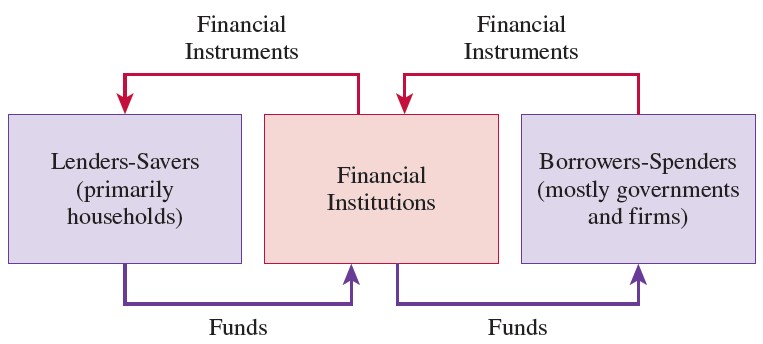
The financial system channels funds from lenders to borrowers through intermediaries.
- In indirect finance, a financial institution takes the resources from the lender and then provides them to the borrower in the form of a loan (or the equivalent).
- With direct finance an agent can invest in a firm directly (buying stock).
What other roles of Financial System
- Channel Saving to investor
- Redistribute Risks
- Information related roles
- Design related reasons
Unit 2.2:The Government and Financial Markets
Why do goverments invest?
- Redistribute the consumption of the stream of income (timing of consumption). Government does not want to maximize profits (at least not always) but rather they want to maximize the wefare of everyone in the economy (This means investment in education, infrastructure, health system etc).
The Government Spending Multiplier
Equilibrium in the Market for Goods and Services is represented by:
- $t$ : taxes
- $r$ : interest rate
- $X$ : export
- $M$ : import
- $e$ : exchange rate
Take $I$, $X$ and $M$ to be exogenous for now. Then the government purchases multiplier is:
Which is greater than 1 if $\partial C/\partial Y \in (0,1)$
Government spending is worthwhile if the increase in output is more than the increased interest cost.
Government expenditure would yield higher returns by increasing aggregate output in the future, which could make the cost of borrowing worthwhile.
- Health
- Education (Human Capital)
- Infrastructure
- R&D
A little model of government and debt
Assume that the governments is running a balanced budget and that at t = 0, the government runs a one-off deficit by issuing one-period bonds:
Let the governments run a balanced budget from t =1 forever, that is:
- Keeping Books Balance : Tax revenue = government expenditure
Suppose that:
- The growth of taxes and expenditures is a constant, $g$.
- Think of $g$ as the rate of growth of the economy.
- Also, that the interest rate on government debt is a constant, $r$.
If the government continues to run a balanced budget, the debt keeps accumulating:
Similarly, tax revenues (and expenditures) grow
Sustainability of debt
One way to think about the sustainability of the debt is the debt/revenue ratio (upper case gamma):
We will define the growth rate of the debt/revenue ratio (lower case gamma) as:
So, if $g > 0$
- If $r_t>g$,$\gamma_t>0$ - debt burden outpaces growth
- If $r_t<g$,$\gamma_t<0$ - revenues grow faster than debt pile
For a fixed growth rate of the economy (g), the sustainability of debt depends on the interest rate (rt).
The interest rate is determined in Financial Markets.
Moreover, the size of the debt/revenue ratio may influence the interest rate.
- If $r_t>g$, $\Gamma$ keeps growing for a long time, $r_t$ may go up, making the acceleration worse
Unit 2.3:Classifying Financial Markets
In terms of the broad type of financial instrument that is traded we can divide financial markets in the following categories:
- Deposit-Loan market
- Money market
- Securities (bond and equity) markets
- Derivatives market
- Foreign exchange market
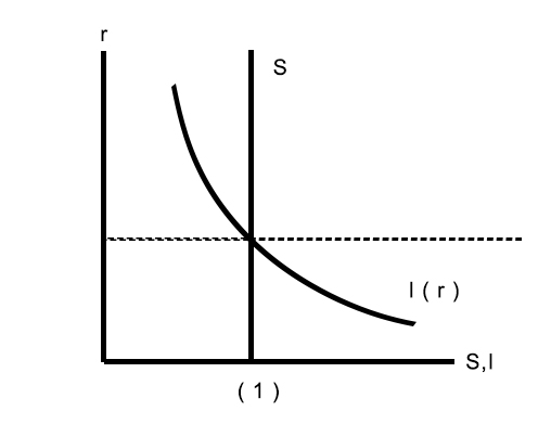
(1) Deposit-Loan Market
Implicitly this market assumes a framework described by the following forces:
- A demand for loanable funds by those with a spending deficit.
- A supply of loanable funds by those who wish to obtain some return on surplus funds (made available through different instruments).
Where there is an imbalance between demand and supply, prices adjust to reestablish the equilibrium. Prices in this context are interest rates.
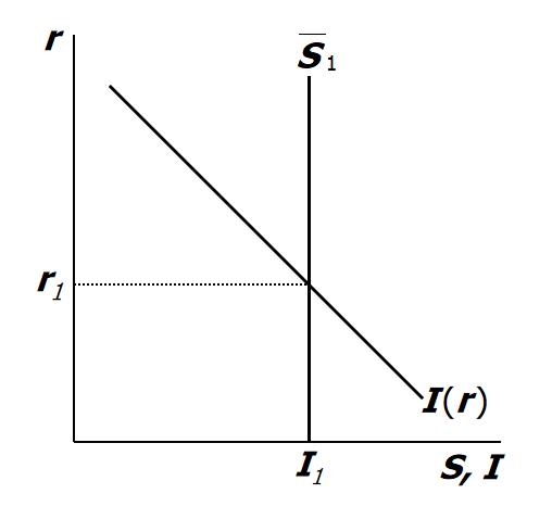
- Demand for loanable funds is planned investment, I(r), which is negatively related to the real interest rate r.
- Supply of loanable funds is national savings, S(Y) which we assume are not affected by r, but which increases with Y since $S = Y - C - T$ (assuming G = T ) or $S = ( Y - T - C ) + ( T - G ) =$ private savings + government savings
Then if $S = I(r)$, the schedule also gives us all points at which the goods market is in equilibrium:
The IS curve gives combinations of r and Y such at Investment (I) = Savings (S). Hence its name, IS curve.
(2) Money Market
The Money Market is for short term funds.
This market clears (short term) surpluses and deficits among financial institutions.
In the traditional money market, banks are linked indirectly through the Central Bank’s automated clearing house (ACM).
- At the end of the day, all these transactions are cleared in the automated clearinghouse in the central bank.
- And the corresponding balances are transferred between banks.
Inter-bank money market connect banks directly.
- lending money to other banks
Central Bank transmits interest rate signals through the money market.
(3) Security (Bond and Equity) Markets
- Primary markets for bonds and equity enable long term funding.
- Companies issue equity and (corporate) bonds to finance their projects and expansions.
- The government issues (government) bonds to finance its budget deficit.
- Secondary markets for equity and bonds.
- Provide liquidity.
- Allow the values of shares and bonds to adjust according to demand and supply.
(4) Derivatives Market
A derivative is a financial instrument whose value depends on (is derived from) the value of some other financial instrument, known as the underlying asset.
- Derivatives help us to hedge (or speculate) against price movements in underlying assets.
- There are many examples, including:
- Forwards – private agreement to exchange at future date and price.
- Futures – standardized forward contracts traded in organized exchanges.
- Options – give the owner the right to buy (or sell) a financial instrument in the future at some specified price.
- Swaps – contracts that allow traders to transfer risk by exchanging financial instruments or cash flows in the future.
(5) Foreign Exchange (Forex) Market
Foreign currencies are exchanged when goods and services are exported/imported and when capital flows across borders.
- The Forex market also allows foreign currency trading.
- Profits from arbitrage opportunities and speculation around future currency values.
- In the Forex market, the price of a currency is expressed in terms of another currency (exchange rates).
- Forex markets are driven by the demand and supply of foreign currencies.
- If exchange rates are floating, the price is determined by market forces
- Some currencies are pegged (tied) to another. Or governments may intervene to affect market exchange rates.
Unit 2.4:The Loanable Funds Model for a Small Open Economy
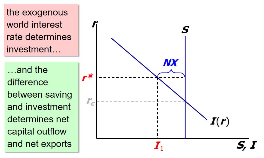
The exchange rate and fundamentals
- $NX = X -M$
- $S = Y - C - G$
so we have
- $S - I = NX$
- If $S - I > 0$ then $NX > 0$, we have a trade surplus
- China, Germany are big savers, and have big trade surpluses.
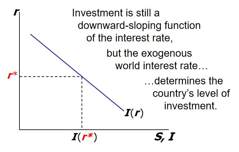
Assumption: Small open economy with perfect capital mobility.
- His implies that the domestic interest rate, r end up aligned to the world interest rate, r (r = r).
- Under perfect capital mobility, any discrepancy between the domestic and the world interest rate triggers capital movements restoring the parity.
Revisiting the demand for loanable funds (small open economy)
The Nominal Exchange Rate
e = nominal exchange rate, the relative price of domestic currency in terms of foreign currency (以外币为单位)
The Real Exchange Rate
$\epsilon$ = real exchange rate, the relative price of domestic goods in terms of foreign goods (e.g., German cars per British car)
- P : Domestic level of prices
- P* : Level of prices in abroad
In the real world: We can think of $\epsilon$ as the relative price of a basket of domestic goods in terms of a basket of foreign goods.
In our macro model: There’s just one good, “output.” So $\epsilon$ is the relative price of one country’s output in terms of the other country’s output
How $\epsilon$ is determined (If $\uparrow \epsilon$ )
- $\Rightarrow$ domestic goods become more expensive relative to foreign goods
- $\Rightarrow \downarrow X,\uparrow M$
- $\Rightarrow \downarrow NX$
Effects of Fiscal Policy in the Home Country
$\downarrow S=Y-C-\uparrow G$
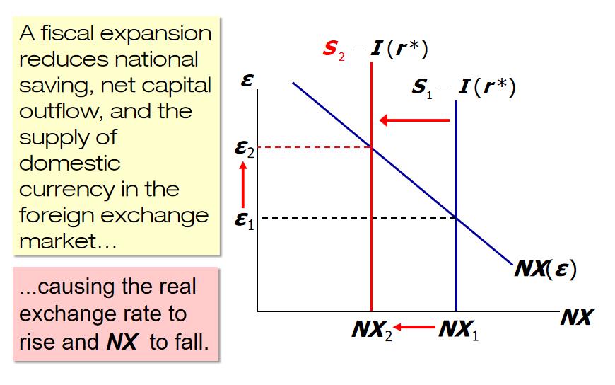
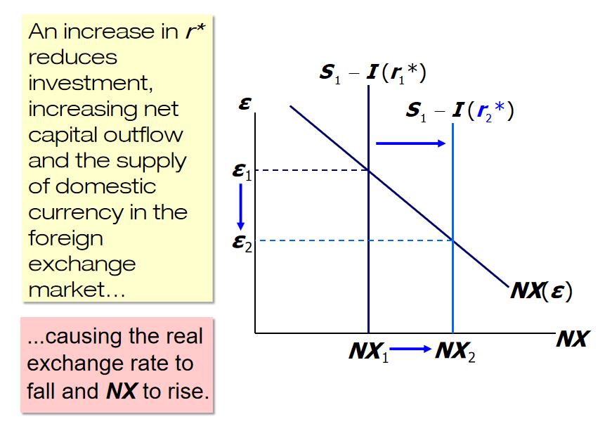
Effects of Fiscal Policy Abroad
Topic 3 – Interest Rate Determination: The IS-LM model
Supplementary Reading
Mankiw, N.G., Macroeconomics (2007, 2010, 2013, 2015, 2018), Ch. 11, 12 & 14
Unit 3.1:The Short Run: The IS and LM curves and the model equilibrium
在此部分 M 不代表进口,代表 money supply
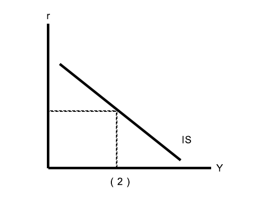
The IS curve
(a) The loanable funds model with (b) The IS curve
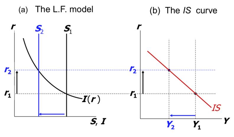
$ \downarrow S=\downarrow Y-C-G$ and $\uparrow r$
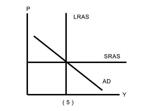
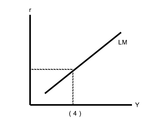
The LM curve
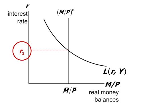
The Market for Money and the Theory of Liquidity Preference
A simple theory in which the interest rate is determined by money supply and money demand. —- John Maynard Keynes
The supply of real money balances is fixed:
where
- The price level $P=\bar{P}$ is fixed in the short run
- The money supply $M=\bar{M}$ is an exogenous policy variable
The demand of real money balances is a function of the real interest rate and income:
where we assume that
- $\frac{\partial L}{\partial r}<0$ - higher rates mean less money demand
- Interest rate is opportunity cost of holding liquid assets (e.g., cash).
- $\frac{\partial L}{\partial Y}>0$ - higher income means more money demand
Money Market Equilibrium
Money market equilibrium, $(\frac{M}{P})^d=(\frac{M}{P})^s$
For a given Y, the euqilibrium interest rate is that which equates supply and demand:
The LM curve is a graph of all combinations of r and Y that equate the supply and demand for real money balances.
The equation for the LM curve is:
Deriving the LM curve
(a) The market for real money balances (b) The LM curve
Since the supply of real money balances is fixed, there is now excess demand in the money market.
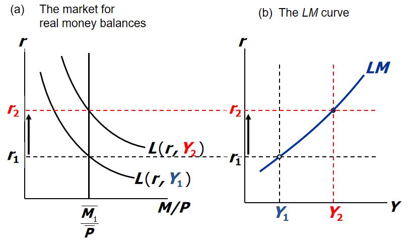
r,Y 成反比,为了保持 L 不变,Y 增加 r 增加,线增高
What happens if Money Supply M is reduced?
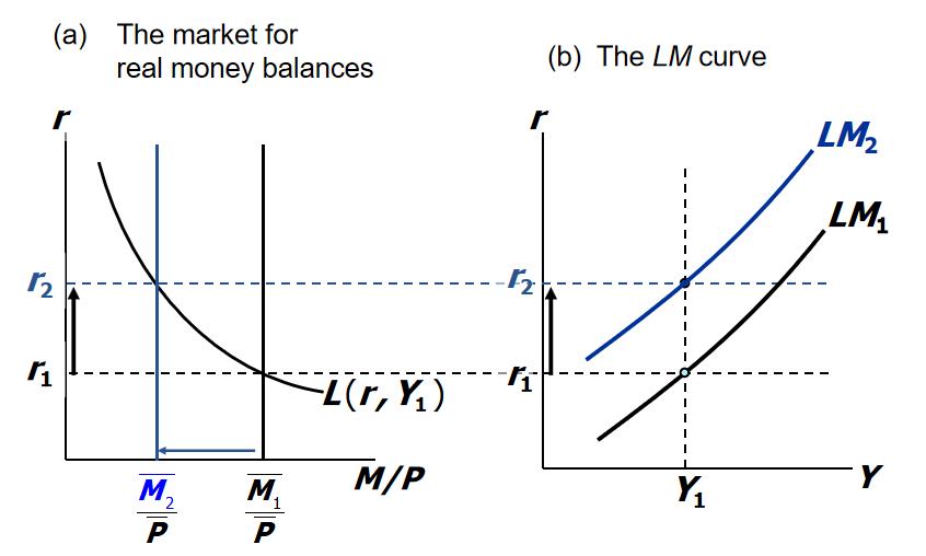
The hidden market in the IS-LM model
The IS represents equilibrium in the goods market($Y\uparrow,r \downarrow$) and the LM equilibrium in the money market($Y\uparrow,r \uparrow$).
But there is a third market in the model – the market for bonds.
- Walras’ Law says that if we have N markets, and N–1 are in equilibrium, then the Nth market must also be in equilibrium.
The reduction in M comes about through OMOs (open market operations)
- The central bank sells government bonds on the open market.
- The buyers of the bonds pay with cash, reducing the money supply.
- Effectively the government is increasing the supply of bonds in the market (reducing the money supply $(\frac{M}{P})^s$). This reduces the price and increases the yield of bonds ($r \uparrow$).
Bond Prices and Yield
where $\bar{P}\to E[Inflation]=0$
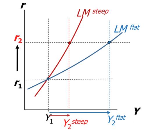
What determines the slope of the LM?
- The slope of the LM curve is determined by how sensitive is the demand for money to changes in the real interest rate.
- The more sensitive is L(r, Y) to changes in r, the flatter is the LM curve.
- The less sensitive is L(r, Y) to changes in r, the steeper is the LM curve.
The short-run equilibrium
The short-run equilibrium is the combination of r and Y that simultaneously satisfies the equilibrium conditions in the goods and money markets.
Unit 3.2:Fiscal and Monetary Policy in the Short Run
- We can use the IS-LM model to analyse the effects of
- Fiscal policy, G, T
- Monetary policy, M
- We can also think about the short run and long run effects.
- Short run: prices are fixed
- Long run: prices can change
Expansionary monetary policy – increase in M
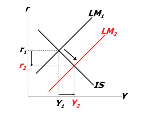
- LM shifts down $\to$ reduces r at original Y
- Once r fall, investment increases by I(r)
- Investment increases causes Y to go up
- Higher Y causes higher S(Y)
Effectiveness of monetary policy
- Slope of the LM
- The less sensitive $M^d$ is to r, the steeper is LM
- Slope of the IS
- The more sensitive I is to r, the flatter the IS curve
- Zero lower bound
- There needs to be room for r to drop. If is already close to zero, it cannot fall further to stimulate the required increase in I
Other factors
- The example is in closed economy. If we open the monetary policy, exchange rate are start to interrupt.
Expansionary fiscal policy
– increase in G, or decrease in T
Recall spending multiplier
IS curve shifts to right by an amount greater than $\Delta G$ if $\frac{\partial C}{\partial Y}\in (0,1)$
- For a given r, higher Y increase money demend
- given $\bar{M}$ and $\bar{P}$, this means a higher interest rate
- Higher interest rate reduce I, depressing Y
- Crowding out (刺激消费)
Effectiveness of fiscal policy
Marginal propensity to consume determines spending multiplier (higher MPC means larger shift to IS)
Slope of IS
Sensitivity of investment to r determines
Determines extent of direct crowding out
Slope of LM
- Sensitivity of money demand to r
- A higher r for equilibrium in money market crowds out more investment
Other factors
- How easy is it to increase government spending? Cost of borrowing? Resistance to taxes?
Unit 3.3:Using the IS-LM Model to Inform Policy in the Short Run
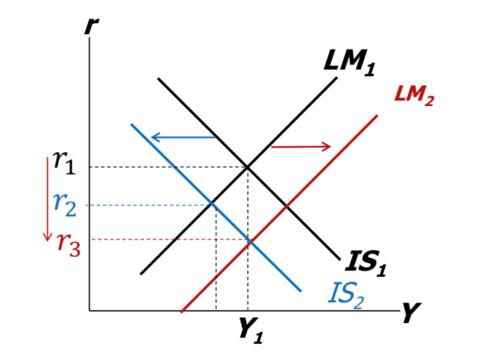
Effect of Shocks on the Economy
LM:shocks to $M^d$
- A wave of credit card fraud increases demand for cash
- Financial innovation, or online shopping reduces demand for cash
- Confidence in the banking industry shifts
IS:shocks to I, C
- Asset price boom that increase consumption
- Increase in business confidence that increase investment
- Inproved consumer confidence
Policy Objectives
- Targeting an interest rate but keep output constant
- Respond to an economic downturn without increasing spending
- Decrease money supply without changing output
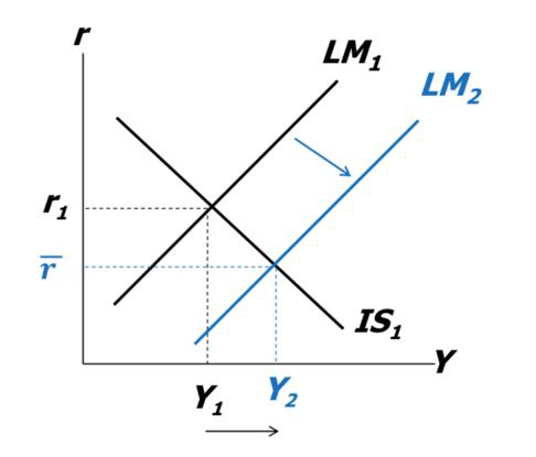
Targeting r
Using monetary policy to reduce interest rate to a target level $\bar{r}$
- CB needs to sufficiently increase $\bar{M}$
- Result also in Y increasing
Response to a demand shock
- Fiscal response to an asset shock that causes Y to fall
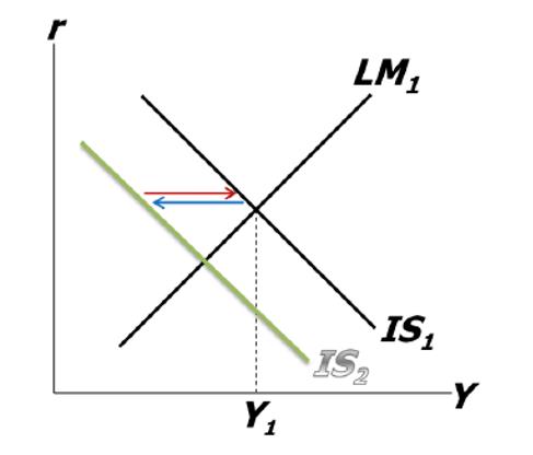
Sometimes fiscal policy may be constrained
Policy makers may not want to use fiscal policy (increase taxes) because of the repercussion on budget deficit
- Expansionary monetary policy restores Y but causes r to fall even further
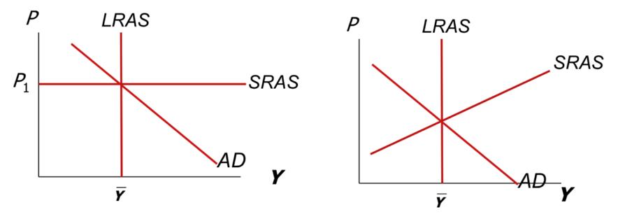
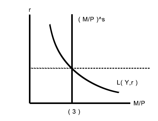
Unit 3.4:The Long Run: The AD and AS curves and the model equilibrium
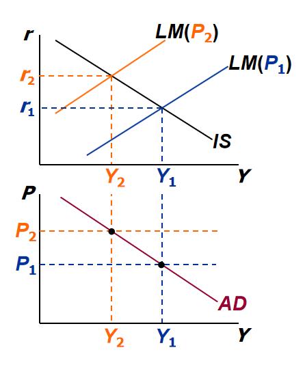
Aggregate Demand (AD)
- Increase in P causes a fall in real money balances
Deriving the AD curve
- $\uparrow P\Rightarrow\downarrow(M/P)\Rightarrow LM shifts left\Rightarrow\uparrow r\Rightarrow\downarrow I\Rightarrow\downarrow Y$
Aggregate Supply (AS)
The short-run Aggregate Supply (SRAS) curve
- P is either fixed or moves slowly
- Output can fluctuate around its full employment level ($\bar{Y}$)
The long-run Aggregate Supply (LRAS) curve
- Captures the long run Aggregate Supply where the price level P varies to achieve full employment level $\bar{Y}$
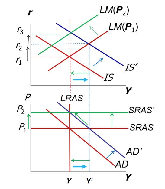
Expansionary fiscal policy in the short and long run
– increase in G
Starting from $\bar{Y}$. Short run
- IS shifts to right
- AD shifts to right
- P is fixed, so output increases to $Y>\bar{Y}$
Over time
- Because $Y’>\bar{Y}$, prices go up
- SRAS shifts up
- Movement along AD by real money balances declining (LM shifts left)
Long run outcome
- Output returns to $\bar{Y}$
- Prices now higher
- Interest rates higher (all of increase in G reduces I)
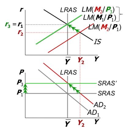
Expansionary monetary policy in the short and long run
– increase in M
Short run
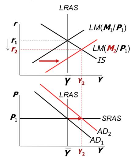
$Y_2>\bar{Y}\Rightarrow\uparrow P$
Long run
Topic 2-3 总结
定义
- Y : GDP
- C ( Y , t ) : Consumption
- I ( Y , r ) : Investment
- G : Government purchases
- NX : Net Exports
- X : Export
- M ( Y , e ) : Import
- $\bar{M}$ : Money supply
- P : Price
- S ( Y ) : Saving/ Supply of loanable Funds
- L ( Y , r ) : Demand of real money
- T/t : Taxes
- r : Interest rate
- e : Exchange rate
- $\epsilon$ : Real Exchange rate
Expansionary Fiscal Policy : $T\downarrow G\uparrow$
Expansionary monetary Policy : $M\uparrow$
Demand Shock $\to$ Price boom $\to$ $C\uparrow$
 |
 |
|---|---|
 |
|
 |
 |
|
(1)$Y\uparrow$,S右移;
(1)S左移,$r\uparrow$;
(2)$r\uparrow$,IS中$Y\downarrow$;
(1)S中非Y变换会导致它偏移;
(3)$Y\uparrow$,L(Y,r) 右移;
(3)L(Y,r)右移,$r\uparrow$;
(4)$r\uparrow$,LM中$Y\uparrow$;
(3/4)$\frac{\bar{M}}{\bar{P}}$左移,$r\uparrow$,此时考虑L(Y,r)不变,即Y不变,LM左移;
(5)$Y\uparrow$, 短时AD右移,过度SRAS上移,长时$Y$恢复$P\uparrow r\uparrow\uparrow$;
Topic 4 – Money and Interest Rates in an OLG model
Supplementary Reading
For a standard exposition of the OLG model see:
- Romer, D., Advanced Macroeconomics, Ch. 2 (2006, 2011 or 2017).
More advanced, but closer to our discussion:
- Blanchard and Fischer (1989) Lectures in Macroeconomic, MIT Press, Sections 4.1 and 5.2.
相似的有 耶鲁大学:金融理论 讲了费雪的不耐定理和用养老保险金为例子讲了世代交叠模型
Unit 4.1:The Economy as an Overlapping Generations of Agents
In the last couple of weeks we have looked at models that were based on macroeconomic variables.
This week we look at interest rates here as a result of preferences and interesting generational dynamics.
A Simple OLG Model
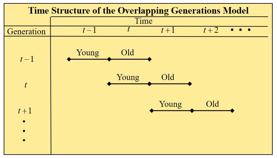
We assume there is a single commodity which is perishable. (Can not be conserve)
An OLG set-up thus brings useful features
- Life-cycle dynamics, interfenerational features
- Savings and investment
- A role for fiat money
Endowments and Consumption
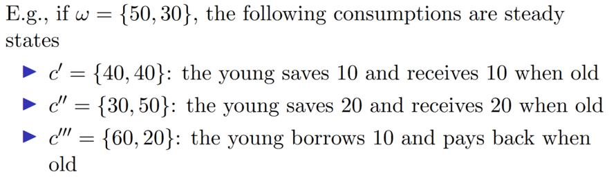
Each generation born at t will receive an endowment $\omega_y$ when young and $\omega_o$ when old
- There is no other form of producing the consumption good
- The endowment cannot be stored or transferred
| Agents born in generation t | Endowment (Wealth) | Consumption |
|---|---|---|
| Young | $\omega_y$ | $c_y$ |
| Old | $\omega_o$ | $c_o$ |
The simplest type of equilibrium:
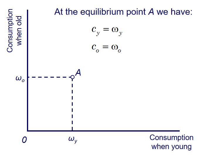
If agents would be able to save
- Savings opportunity exist at 5% interest rate.
- Agents would like to ‘smooth’ their consumption.
If the endowments are the following
And assuming agents save 1/4 of their endowment when young
Unit 4.2:Preferences, Interest Rates and Optimization
Agents maximize their lifetime utility subject to their lifetime budget constraint
- Lifetime utility
- Lifetime budget constraint
(Present Value of Consumption = Present Value of Wealth)
Indifference Curves (无差异曲线)
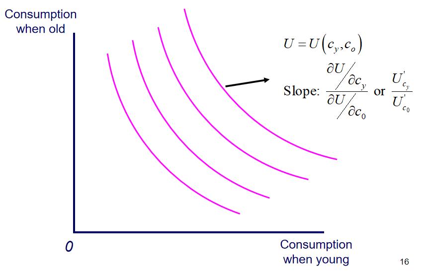
Shape and position of indifference curves indicate consumer preferences
Movements onto higher indifference curves indicate higher utility
同一条线上 Utility 相同,越高越好
If an agent decide to save all his/her endowment when young
Or he/she borrow his/her endowment when old and consume all when young
The Lifetime Budget Constraint
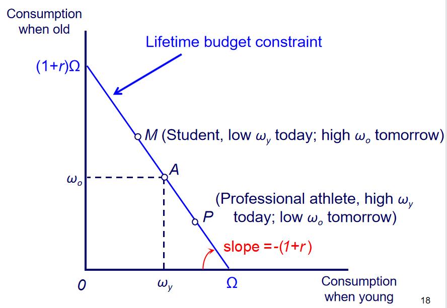
Optimal consumption: borrower
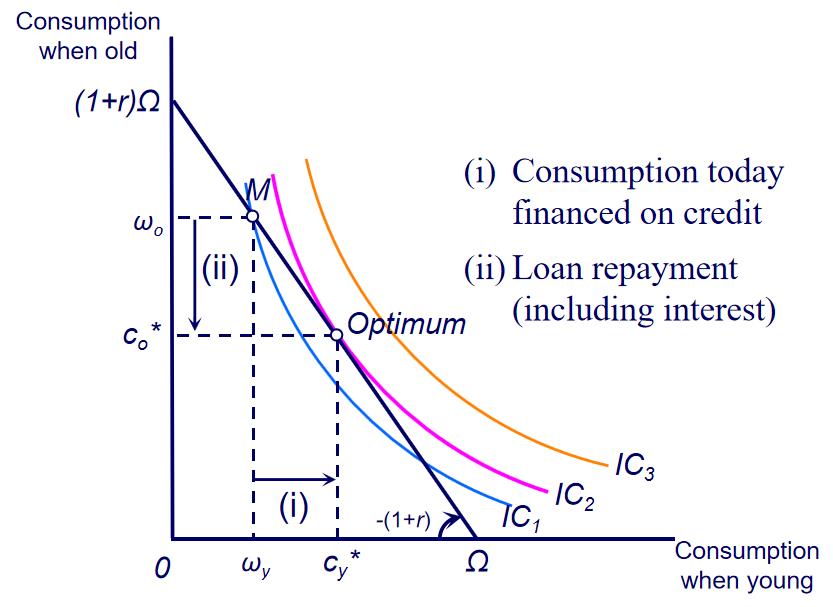
低收益的学生可以通过贷款让C达到更高的U
Optimal consumption: saver
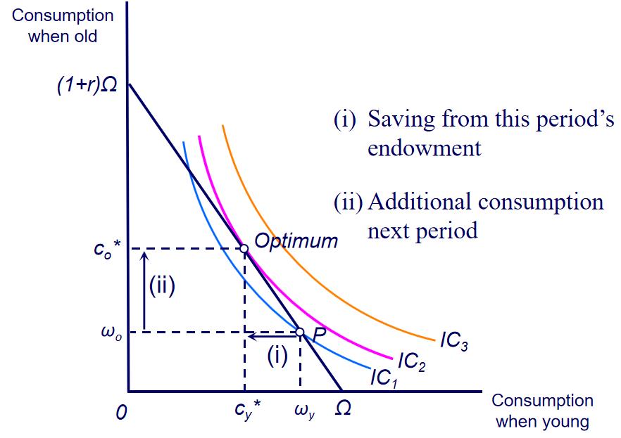
高收益的教授可以通过存款让C达到更高的U
The Consumer’s Optimization Problem
Maximise lifetime utility subject to the lifetime budget constraint:
Notice that we can also write this problem as:
用这个式子直接代入用 s 消掉 c,然后对 s 直接求导也是可以的
In this setting, $\omega_y,\omega_o$ and $r$ are all exogenous
Solving for $c_o$ in the lifetime budget constraint we have:
and then substitute for $C_o$ in the utility function
After some maths,
optimal consumption when young is
and since $s=\omega_y-c_y$, we can see that $r\uparrow$ means $s\uparrow$
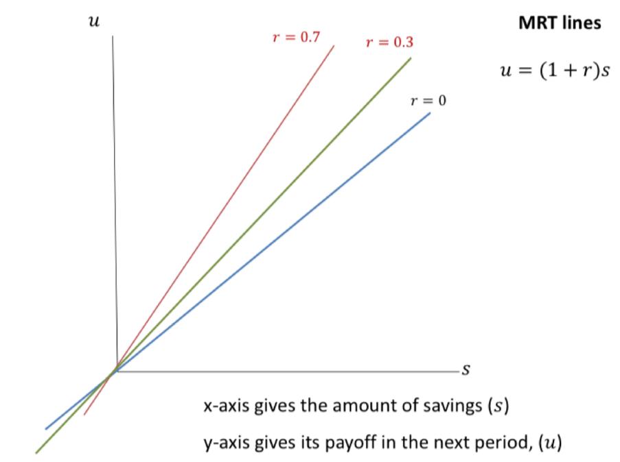
Unit 4.3:Interest Rate Determination
This is the marginal rate of transformation (MRT)
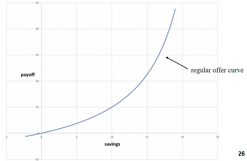
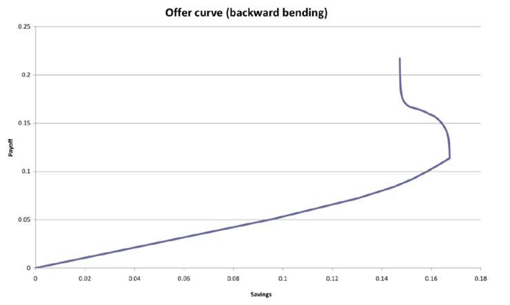
The offer curve (based on preferences)
考虑了价值
Features of a regular offer curve
- Crosses origin
- Upward sloping
This is a combination of two effect
- Substitution effect
- When r increases, $c_o$ become ‘cheaper’ (rather than consum when young - oppotunity cost)(以后的东西更加便宜)
- Income effect
- When r increases, saving will earn more so the agent can save less and increase both $c_y$ and $c_o$ (总资产增加)
Combination
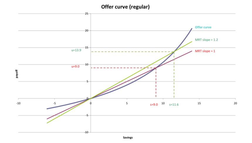
- In a regular offer curve, the substitution effect dominates the income effect, so saving increase in interest rate
- If the income effect dominates at some level of interest, we can have a backward sloping offer curve
The steady state
A steady state equilibrium is one that is stable over time. All agents face the same problem, so perhaps they always consume and save the same amounts.
For each of these steady state allocations require a 0% interest rate for each generation to behave the same
The optimal point at intersection point
Unit 4.4:Adding Money to the Model
Solving the issue of the saving-payoff transfer by introducing ‘bits’ of paper
- Intrinsically worthless bits of paper
- It is liquid and tradeable
- They can exchange it and it can imply a price of goods
- Price of goods is supply of money divided by quantity of goods traded
A feature of the OLG model with money is that it can have many equilibria. We can also find the non-steady state equilibria (optimal but prices changing).
Consider point B on the offer curve
- $s=8.3, u=7.9$
- $p_{t=0}=1/8.3=0.1205$
- $p_{t=1}=1/7.9=0.1261$
What is happing to price over time
If $r<0$
- $s\downarrow, u\downarrow, p\uparrow$
- r通常为正
Topic 5 – Determinants of Firm Value (Part I):Present Value, Competition and Monopoly
Supplementary Reading
For the corporate finance aspects of the lecture see:
- Hillier, D., Ross, S., Westerfield, R., Jaffe, J., Jordan, B. (2020) Corporate Finance, 4th Edition, McGraw Hill, Ch. 5.
For the economics aspects of the lecture see:
- Mankiw, N.G., Taylor, M.P (2020) Economics, 5th Edition, CENGAGE, Ch. 10-11.
Unit 5.1:Bond Valuation
Securities issued by corporations can be roughly classified as equity securities (stocks) and debt securities (bonds).
From a financial point of view the main differences between equity and debt are the following:
Debt is not an ownership interest in the firm. In contrast, if you buy equity (by definition) you are getting a portion of the company.
The corporation’s payment of interest on debt is considered a cost of doing business, and is fully tax-deductible. Dividends paid to shareholders are not deductible.
就相当于,debt是对于外部的欠款,需要计入账中。Shareholders相当于自己人,内部分红
Unpaid debt is a liability of the firm. If it is not paid, creditors can legally claim the assets of the firm. This possibility does not arise when equity is issued.
bonds 的收益是固定的,而 stocks 因为贬值而没有分红是正常的
What is a Bond?
A bond is a fixed-income security that is issued in connection with a borrowing (or debt) arrangement.
Some important terms:
Coupon Payments ( C ): flow of interest payments (bond payoffs).
Face value (or par value) ( 100 ): Principal amount of the bond at maturity.
Coupon rate: Percentage of the face value that is paid as coupon payment.
Maturity ( T ) : The specified date on which the principal amount of a bond is paid.
Yield to maturity (YTM) ( r ) : The rate required in the market on a bond. It is expressed in annual terms.
通常是名义利率
实际=名义-通货膨胀
Bond Value Formula
- $\uparrow r\Rightarrow \downarrow Value$
Unit 5.2:The Not-So-Easy Task of Finding the Value of a Stock
What is a Stock?
A stock is a share in the ownership of a corporation. It represents a claim on the company’s assets and earnings. There are two types: ordinary equity and preference shares.
- Ordinary Equity (普通股)
- Equity without priority for dividends, or in a bankruptcy
- Preference Shares (优先股)
- Equity with dividend priority over ordinary stocks, normally with a fixed dividend rate, normally without voting rights.
The Cash Flow Model
We need to calculate to present value of the future cash flows of a stock to find its price.
Unfortunately, this is not straightforward for the following reasons:
- We do not know the future cash flows of a stock.
- In bond valuation we know the coupon payments and face value.
- In theory, a stock can last forever, we do not know the life of the investment
- In bond valuation, time to maturity is given.
- It is not easy to observe the required rate of return in the market.
- In bond valuation, the YTM can be calculated using bond market prices.
Cash Flow Valuation t-periods-holding stock
- The difficulty is knowing the price of the stock in the end period, which is normally not possible.
The Dividend Discount Model
We can extend the cash flow approach for an infinite stream of dividends and no future final sale price.
Unit 5.3:Special Cases of the Dividend Discount Model
Dividends with Zero-Growth
We have already seen this case when we studied ordinary perpetuities
Dividends with Constant-Growth (g)
We have also seen this case when we studied growing perpetuities
Dividends with Non-Constant Growth
Where does “g” come from?
Dividing by Earnings this year both sides
Where does “r” come from?
Dividend Yield
- Expected cash dividend divided by its current price
Capital Gains
- Expected Stock price Appreciation
Dividends vs. Capital Gains
The value of an equity is £100. The company earns £100 extra in cash. What is the investor’s portfolio at t =1?
| 100% Dividends | 0% Dividends | 50% Dividends |
|---|---|---|
| $P_1$ = £100 | $P_1$ = £200 | $P_1$ = £150 |
| g = 0 | g = 1 | g = 1/2 |
| $D_1$ = £100 | $D_1$ = £0 | $D_1$ = £50 |
| Total = £200 | Total = £200 | Total = £200 |
| Dividend Yield = 1 | Dividend Yield = 0 | Dividend Yield = 1/2 |
r = (£200 - £100)/£100 = 1 = Dividend Yield + g
Unit 5.4:The Value of the Firm
Growth Opportunities
Cash Cows vs. Growing Companie
Earnings per share (EPS) can be split into dividends (DPS) and retained earnings
100% Dividends
- EPS = DPS
- Share price = EPS/r = DPS/r
- Value of the firm without any additional reinvestment
0% Dividends
- All EPS is reinvested in firm
- Dividends = £0
- Share price = EPS/r + NPVGO
- NPVGO = Net Present Value of growing opportunities
The Price–Earnings (P/E) Ratio
Dividing by EPS both sides
The P/E ratio is based on the idea that the absolute value of a stock is not as important as its relative value.
The P/E ratio measures how much investors are willing to pay per unit of current earnings.
Companies with high growth opportunities will have higher P/E ratios.
- Be careful though, we are not only looking at the stock price here, but also at earnings per share. A high P/E may also result from low earning per share (denominator effect).
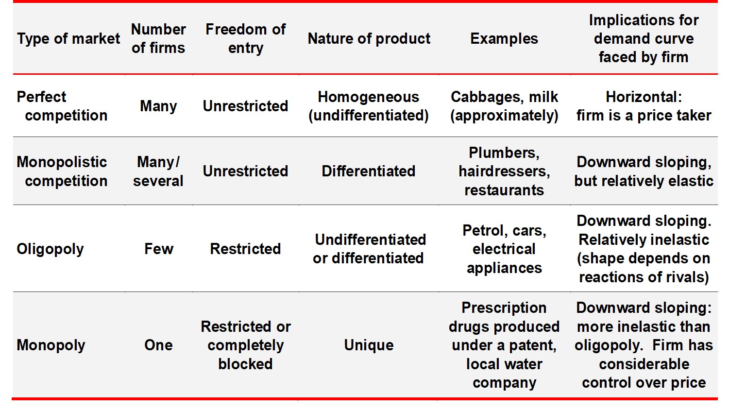
Unit 5.5:Market Structures and Earnings
Market structures are classified by level of competition
The degree of competition is determined by the following factors:
- Number of firms
- Freedom of entry to the industry
- Nature of the product
- Nature of the demand curve
The four market structures are:
- Perfect competition
- Monopolistic competition
- Oligopoly
- duopoly
- Monopoly
Monopoly Power
A firm can exert monopoly power by charging a price above marginal cost.
- Monopoly power can be exerted even if the firm does not control the whole market.
Governments attempt to control or curb monopoly power.
Monopoly power allows companies to have excess profits.
The Fundamental Cause of Monopoly: Barriers to Entry
- Ownership of key resources
- When a single firm is the owner of a key resource.
- Government-created monopolies
- Patent and copyright laws create monopoly power but are crucial for innovation.
- Economies of scale
- Natural monopolies take advantage of economies of scale.
- Arise when a single firm can supply a good or service to the entire market at a lower cost than two or more firms could.
- Horizontal integration
- Acquisition, merger or takeover, leading to the industry being more concentrated.
Topic 6 – Determinants of Firm Value (Part II):Monopolistic Competition
Supplementary Reading
The seminal paper on the area is:
- Dixit and Stiglitz (1977) Monopolistic Competition and Optimum Product Diversity, American Economic Review, 67(3), 297-308. Available here:
For a “lighter” version see:
- Dinger (2009) The basics of “Dixit-Stiglitz lite”, teaching notes. Available here:
Unit 6.1:What is Monopolistic Competition?
Monopolistic competition: A market structure in which many firms sell products that are similar but not identical.
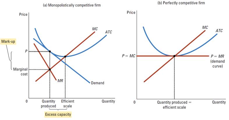
- MC:Marginal Cost
- MR:Marginal Revenue
- ATC:Average Total Cost
- Profit = ( Price - ATC ) * Quantity
MC 通过 ATC 最低点
MR 在垄断企业通常比 Demand 小
Only the perfectly competitive firm produces at the efficient scale.
Price equals marginal cost under perfect competition, but price is above marginal cost under monopolistic competition so exerting market power.
Unit 6.2:Structure of the Dixit-Stiglitz Model
目的是平衡多样性带来的垄断利益,和大规模生产带来的低平均花销
Firms
There are two types good firms
- Intermediate good firms
- Monopoly producers of unique, differentiated products
- Hire labour and capital as inputs
- Free entry to being a producer of a different variety
- Individual producer has some market power
- Final good firms
- Use intermefiate goods to produce a final consumption good
- For the final goods producers, the intermediate inputs are imperfect substitutes
- Final good is sold in a perfectly competitive market - individual producers have no market power
Unit 6.3:Intermediate Goods Producers
There are $N$ firms producing different outputs $q_n$ using capital $k$ and labour $l$,
- $\theta_n>0$ is the individual firm’s productivity
- $\gamma$ is the share spent on capital, which we assume is common to all firms
Profit Maximization
Each of the $N$ monopolists maximise their own profits by choosing
- How much to produce, $q_n$
- What price to charge, $p_n$
- choice of $q_n$ affects the price $p_n$
- How much labour and capital to use in production
Unit Cost Function for Each Firm
In order to minimizes its cost of production, taking $w$ and $r$ as given
- $w$:wage
- $r$:rate
We can writed down capital as a function of labour and output
So we have costs as
For a given level of output, the cost-minimizing amount of labour is found by
The optimal choice of labour as a function of input prices ($r,w$), output level ($q$) and technological parameters ($\theta$):
- Higher $r$ (or lower $w$) means that more labour is used
- More output means more labour required
- For a given level of output, more productive firms need less labour
Substituting $l_n^*$ into equation, we obtain optimal choice of capital,
- Higher $w$ (or lower $r$) means that more capital is used
- More output means more capital required
- For a given level of output, more productive firms need less capital
Put these into cost function, we have cost as a function of output level.
which becomes
The ‘unit cost’, the cost of producing one unit of output, for firm $n$ is thus,
一单位最小花销
推导过程其实有点问题,因为不能保证 labour 的最优就是 capital 的最优,导致最终公式的边际值是稳定的,只能猜测这里采用了理想化的方法
Unit 6.4:Final Goods Producers
Production Function
Final goods $Y$ are produced in perfectly competitive markets by firms that use the following production function,
This is what is called a CES (constant elasticity of substitution) production function
$\sigma=\frac1{1-\rho}$ is the elasticity of substitution between the different $q_n$
- With $\rho\to 0$, this is a Cobb-Douglas (unit elasticity) - 1
- For $\rho\to 1$, the $q_n$ are perfect substitutes (linear) - q 之和
- For $\rho\to -\infty$, the $q_n$ are perfect complements (Leontief) - 趋向 0
substitutes 替代
complements 互补,存在消费依存
总产出(需求) Y 不变,如果 $\rho$ 大,多为替代品,需要的 q 就少,商家间的竞争就大
We focus on $\rho\in(0,1)$, where $q_n$ are substitutes (but not perfectly so)
Profit Maximization and the Demand for Intermediate Goods
Final good producers maximise their profits, given prices of intermediate goods and price of final output $P$,
Marshallian demand for each good
- Downward sloping in $p_n$
- But less downward sloping in $p_n$, the less substitutable the goods are (lower $\rho$)
- Lower as $N$ increases, higher as $Y$ increases
市场由每家生产价格决定每家最优生产产量
Unit 6.5:Optimization, Market Shares, and Profits of Intermediate Goods Producers
Intermediate goods firm optimization
Intermediate good firms maximise their own profits by choosing prices, $p_n$, taking $P,Y$ and $N$ as given, and taking into account the effect on the demand for their good, $q_n^*(p_n)$
Optimal price satisfies,
After some algebra (find $\frac{\partial q_n^*}{\partial p_n}$ first), we have the following:
每家由单位花销决定最优单位生产价格
现在可以由单位(最低)花销->单位价格-> Y & P & q
Note:
- With $\rho\in (0,1)$ this implies some markup in the price over unit cost (额外收益)
- The lower is $\rho$, the less substitutable the goods, the higher the markups
Recall that $C_n^1=\frac{1}{\theta_n}[\frac{r^\gamma w^{1-\gamma}}{\gamma^\gamma(1-\gamma)^{1-\gamma}}]$
- So price is decreasing (and sell more) in firm technology $\theta_n \uparrow$ more productive
Aggregates
The final good can also be written in aggregate as a function of all the inputs (because of constant returns):
where $\bar K=\sum_{n=1}^N k_n$ and $\bar L=\sum_{n=1}^N l_n$ and where $\bar\theta$ is economy-wide average productivity
We can also write down the aggregate price level as,
P 是所有 p 的平均值
Note that we have the price of an intermediate good as,
Both the aggregate price level and individual intermediate firm prices have similar structure
- But the intermediate good firm price can deviate from the aggregate price level (换个 productivity 可以达到从总体到特定生产商价格的转换)
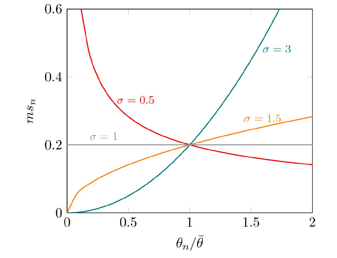
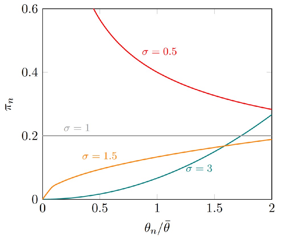
A direct result is to look at market shares of intermediate good firms
Market share (ms) of firm n
- $\sigma=\frac1{1-\rho}$ so $\sigma-1=\frac\rho{1-\rho}$
Observations:
- A firm with average productivity ($\theta_n=\bar\theta$) has market share $ms_n=1/N$
- More productive firms have higher market share (since $\sigma>1$)
- Greater productivety leads to higer market share if goods are more substitutable ($\sigma$ higher)
- A more monopolistic market ($\downarrow \sigma$) protects less productive firms from some competition (保护新生企业,如下图 0.5)
$\frac{\theta_n}{\bar\theta}$: relative productivety of firm
Example:
Market share if N = 5
Profit of firm n
Profit shares behave the same as market shares
Let aggregate profit be,
And firm n profit is aggregate times the market share,
What determines individual firm earnings?
- Macroeconomics: the size of nominal aggregate output (PY-GDP)
- Aggregate market structure: the more competitive ($\sigma$ higher), the less aggregate profit; the more firms, the less share of aggregate profit (N)
- Firm specifics: the more competitive ($\sigma$ higher), the more firms benefit from being productive relative to average ($\theta$)
Example:
Firm profits if N = 5 and PY = 1
当 $\rho<0, \sigma<1$ 时,需要等待低生产的生产同步,导致高生产收益低
Unit 6.4:Earnings and Firm Valuation
Earnings of firm n
Now we have a better idea of what determines earnings, we can return to valuations based on that
Now we have an income syream:
Can we calculate PV based on this?
Firm Valuation
Consider discount factor $\beta=\frac1{1+r}\in(0,1)$, then
where $E_t[·]$ are expectations formed at time t
Suppose that macroeconomic and market factors are forecasted accurately, then uncertainty rests on expectations of firm productivity,
Recall also that $Y(t)=\bar\theta\bar K(t)^\gamma\bar L(t)^{1-\gamma}$
- Business cycle: Positive shock to business cycle (higher $Y(t+\gamma)$ for some $\tau$) means higher firm valuation
- Uncertainty: Future productivity relative to market
- Future market structure: Entrants to market in future lower today’s present valuation
- We would not normally think of $\sigma$ as a time-varying parameter
- More monopolistic market reduces the potential future gains to being more productive
The Long Run
Excess profits attract new entrants
- $N(t)$ going up over time in the future
- With everything else the same, that lowers profits in future
- That means firm valuation is lower today
There are still markups, since prices are not a function of N
From an efficiency perspective
- Prices are higher and output is lower than under perfect competition ($\rho\to 1$)
- If prices were made to be lower, more consumption could increase
Indicidual firm productivity still matters to valuations
But as N goes up, so firm profits decline,
Both the monopolistic competitor and the perfect competitor make zero excess profit in the long-run
Innovation and Marketing
Innovation
- Firms can allocate profits to innovation, improving $\theta_n$
Marketing and ‘non-price’ competition -attempts to shift demand curve and make it more inelastic
- The perception of innovation
- The appearance of difference between products
- Reliability, style, safety, taste $\to$ products
Competition
- The structure of markets can fundamentally change with new technologies
- Disruption
- Creative destruction (‘Schumpeterian’ growth)
Omissions and Extensions
- Firms only rented capital
- If they own capital, stream of profits would relate to changes in value of capital
- Labour market
- We assumed a competitive labour market
- If workers are specialized, or if workers are unionized, then there is a monopsony issue
- Government borrowing may compete with firms
- We have seen previously how price of credit needed for expansion may be affected by crowding out
- Financial market distress also
- Other costs
- Fixed costs of operating, costst of innovation, regulatory restrictions,ets.
- International
- Trade, finance, foregin competition/ subsidies
- Networks and cartels
Topic 6 总结
定义
- Outputs: $q$
- Technological parameters/ Productivity: $\theta$
- Capital: $k$
- labour: $l$
- The share spent on capital: $\gamma$
- The share spent on labour: $1-\gamma$
- Price: $p$
- Cost of production: $C(l,k)$
- $w$:wage
- $r$:rate
Final goods: $Y$
Elasticity of substitution: $\sigma=\frac1{1-\rho}$
Final good producers profits: $\Pi$
Price of final output: $P$
- Intermediate good firms profits: $\pi$
- Market share: $ms$
Topic 7 – Determinants of Firm Value (Part III):Tobin’s q theory of investment
Supplementary Reading
For further reading on the topic see:
- Talmain, G., Teaching Notes on Tobin’s q theory of investment.
- Romer, D., Advanced Macroeconomics, Ch. 9 (2006, 2011 or 2017).
- Blanchard, O., Rhee, C., & Summers, L. (1993). The Stock Market, Profit, and Investment. The Quarterly Journal of Economics, 108(1), 115-136. doi:10.2307/2118497
Unit 7.1:Tobin’s q
A firm is just a bundle of assets ($k_t$) that produces value ($v_t$)
Tobin’s q is a particular representation of this:
- The market value is the market capitalization of the firm(stock price*number)
- The book value is the replacement cost of the captial
q 单位 capital 产生的价值
Net investment is the accumulation (or decumulation) of capital
What does the q tell us?
- If $q>1$, the market assesses some value in the firm beyond the measured assets in the company
- If $q<1$, the market may be undervaluing the firm
Investment:
- If $q>1$, the firm can sell shares at a price higher than it costs to put more capital in the firm
- If $q<1$, the firm may do better to buy back some shares from the market, or let its capital depreciate
This interaction between investment and firm value is our focus
Note a distinction:
- Tobin’s q is about the average value of a firm vs its book value
- Investment decisions are made at the margin: A firm buys an extra unit of capital if that yields more value at the margin than the cost of the captial
Renting vs. Owning the Capital
We need to introduce a role for capital that generates insights about firm value
What we will do is take this in three steps:
- Leased(Rent)capital and firm value
- Firms make no profit, have no value
- Owned capital without adjustment costs
- Firm value is always just the capital stock; $q=1$ always
- Owned capital with adjustment costs
- Interesting dynamics of investment and value, where $q\gtrless1$ in transition to steady state
Unit 7.2:Leased Capital and Firm Value
Firms that Lease Capital
Suppose that capital is owned by leasing companies that rent it out to firms
Firms then hire capital and labour to produce according to
where $f$ is a regular production function with constant returns to scale
In a perfectly competitive environment, firms are price takers, choosing $k$ and $l$ to maximize profits, given prices for output, capital and labour,
The first order conditions of this problem imply,
Euler’s Homogeneous Function Theorem
A function $g(x,y)$ that is homogeneous of degree $\lambda$ has the following property,
- This is called Euler’s Homogeneous Function Theorem
A function that has constant returns to scale is homogeneous of degree one ($\lambda=1$), so we can write the following,
Constant Returns to Scale and Profits
Using this,we have the profits of a firm as,
Given the first order conditions $p\frac{\partial f}{\partial l}=w$ and $p\frac{\partial f}{\partial k}=r$ this means,
We saw previously how departing frim the assumption of perfect competition generated insights to value
Today, we instead focus on the role of owned capital
Unit 7.3:Firms that own capital, without adjustment costs
Now, suppose firms own capital (on behalf of their shareholders)
A firm wants to maximize the present discounted value of the future flow of dividends ($c_t$)
- where $u(c_t)$ is the utility of the representative shareholder
Output, dividends and new capital investment
Production arises out of capital holdings (let’s ignore labour for now)
Output is allocated to dividends (consumption of shareholder) or new capital investment, $i_t=y_t-c_t=rk_t-c_t$ (using Euler’s theorem again $f(k_t)=\frac{\partial f}{\partial k_t}k_t$)
So capital accumulation $\dot k_t=i_t$
The “dot” denotes the derivative with respect to time ($dk_t/dt$) and is the continuous time version of $k_{t+1}-k_t$
Note:
- Implicit here is that capital is fungible - capital can costlessly be converted out of forsaken consumption (no adjustment cost)
Arbitrage and the value of the firm
An investor can
- Buy a publicly traded firm for its market capitalization $v_t$
- Or it can buy new capital $k_t$ at the price of the consumption good
Arbitrage makes the two equal, hence,
It is always $q=1$
If a firm has N common shares in the market, a single share in a firm is then just worth $p_t=\frac{v_t}N=\frac{k_t}N$
Share price with no adjustment costs
According to this approach, the price of a share is simply,
What we did before was to relax the assumption that firms are perfectly competitive
- Now we relax the fungibility assumption
Unit 7.4:Firms that own capital, with adjustment costs
Set-up
We have a simplified framework:
- All firms have the same technology
- Produce identical goods
- Produce using only capital $k_t$
So this model is not so useful in telling use about the valuation of individual firms
- For that, see monopolistic competition
What we have here is how both interest rate and a nontrivial aggregate valuation of equity can be understood together
- So something akin (类似) to a stock market index and how it interacts with interest rates over the business cycle
Production
A representative firm’s production function,
Where we have the regular assumptions,
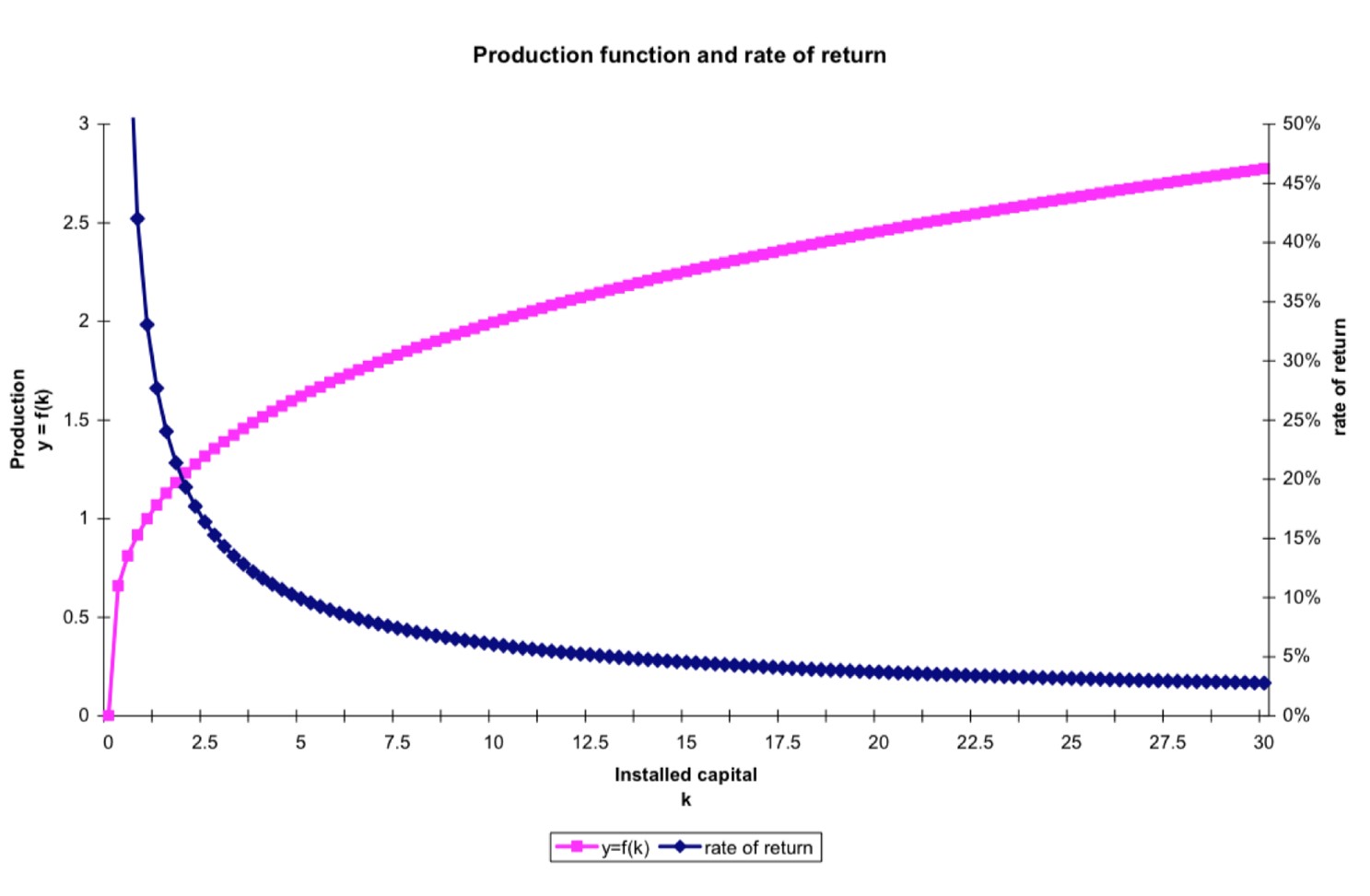
As such, we have a rate of return on capital, $ror_t=f’(k_t)$,
where
Income destinations and the single shareholder in the model
Output at time $t$ can be used in two ways:
- Dividends: to pay $c_t$ to shareholders
- Retained earnings: to invest $i_t$, which leads to:
- Increased capital stock at $t+1,t+2,…$
- Higher production and so, potentially higher $c_{t+1},c_{t+1},…$
We assume all the shareholders share the same preferences
So, without loss of generality we assume there is a single shareholder
Dynamics of Capital and Debt
The firm starts at $t=0$ with an initial stock of captial, $k_0$ and an initial level of debt $b_0$
Out job is to keep track of how these two variables change over time
- Capital accumulation
- Debt accumulation
为了使模型更加灵活,引入 debt
Capital Accumulation
Investment adds to the stock of capital for next period, and we assume (for simplicity) that capital does not depreciate:
Now we want to consider that switching output into capital is not costless
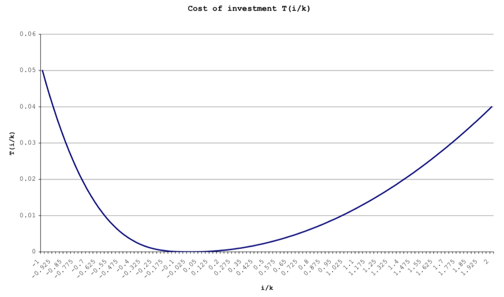
Cost of Installing Capital
For an increase in capital of $i_t$, the firm pays,
The simple cost of the investment $i_t$
Plus cost to install each unit of investment
- where $T$ here is a function of $\frac{i_t}{k_t}$
- We assume $T(0)=0$, $T’>0$ and $T’’>0$
Total cost of capital increase is then,
Note that the firm can also disinvest capital and transform is back into consumption by setting $i_t<0$
Debt Accumulation
In each period $t$, the firm decides how to allocate to investment $i_t$ and dividends $c_t$
- It can finance investment or dividends using retained earnings or debt
- Firm faces interest rate $r_t$
Out of output $y_t$, firm can spend on:
- Dividends $c_t$
- Investment $i_t[1+T(\frac{i_t}{k_t})]$
- Debt interest $r_tb_t$
The level of debt accumulates by the difference between expenditure and income:
Firm Decision Making
The firm can
- distribute more dividends by reducing investment, lowering capital formation and future income
- distribute fewer dividends to increase capital formation and future income
- borrow or lend at the current rate of interest $r_t$ to do more or less of the previous
Hence, many paths for capital accumulation and for dividends are possible
The firm starts with some initial level of capital $k_0$ and debt $b_0$
At time $t=0$ it produces
It uses these earnings to
- Invest in new capital $i_0$
- Pay a cost of installation $i_0·T(\frac{i_t}{k_t})$
- Pay interest on debt $r_0b_0$
- Pay a dividend, $c_0$
The firm’s surplus (or deficit) at the end of period $t=0$ is then,
In the next period, debt will $\downarrow$ by $surplus_0 (+)$
Capital will $\uparrow$ by $i_0$ so $k_1=k_0+i_0$ and production will be,
Out of which it invests, pays on debt, pays dividend, etc.,
Examples of Accumulation Paths
Consider some simple (potentially non-optimal) strategies chosen by the firm:
- Invest if the rate of return on capital is larger than the current interest rate
- Pay dividends to stabilise interest payment : earnings ratio at some level
- I.e., sets some fixed target for $de_t=\frac{r_tb_t}{y_t}=\frac{interest charges}{earnings}$
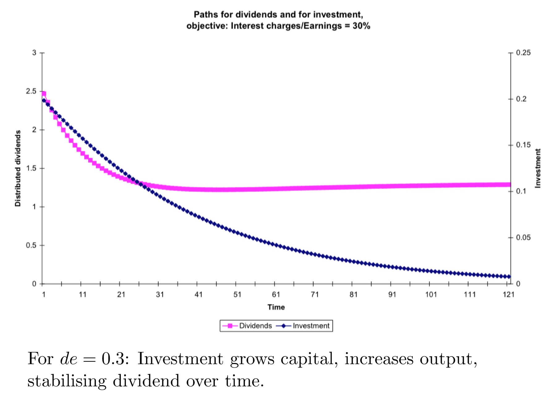
For $de=0.3$: Investment grows capital, increases output, stabilising dividend over time.
For $de=0$: Invest less to avoid debt; accumulate more slowly but increased output is all going to investment and dividend.
Which of these strategies is better?
An intertemporal trade-off:
- In the first case, $de=0.3$, there is a high initial dividend, but lower later
- Where the rule is $de=0$, there is a low initial dividend, but higher later
Which of these is better? Or is there a further alternative that is superior?
We need an objective function for the firm
Unit 7.5:The Shareholder’s Optimisation Problem
Assume that a shareholder’s instantaneous utility is
and that the shareholder discounts future utility at rate $\rho$, then the time $t=0$ present discounted value of future dividends is,
The firm’s objective is to maximise this subject to paths for capital and debt
That is, the firm chooses the dividend stream $\{c_t\}_{t=0}^\infty$ to solve:
subject to
Optimal Paths
What we need to find is the optimal path for dividends and debt
We simplify matters slightly by supposing that $r_t=\bar r$ is constant
The optimality condition, looks like a regular Euler equation:
省略了过程
and since $u(c_t)=ln(c_t)$ this is simply,
Iterating forwards,
- Dividend grows over time if shareholders are patient ($\bar r>\rho$)
- Falls over time if $\bar r<\rho$
We set $\bar r=\rho$ for simplicity
- That means that dividends are constant $c_t=c_0$ along the optimal path
- (Though note we do not know what $c_0$ is yet) $k_0\to c_0,q_0$
The q
Recall that, for the firm, there are two types of capital:
- That which is already installed in the firm
- That which can be installed with unit cost $T(\frac{i_t}{k_t})$
An agent can buy capital to be installed, but it cannot directly buy capital already installed
- What would be the price of an installed unit of capital if such thing was available? — Tobin’s q
Tobin’s q is the value of the capital inthe firm, relative to the value of the capital outside the firm
In other words, $q_t$ is what is called the shadow price of installed capital
Recall
- If $q>1$, then the firm is worth more than the book value of its capital $\to$ investment $i_t>0$
- If $q<1$, the firm is worth less than the book value of its capital $\to$ investment $i_t<0$
Equilibrium stock prices
We can obtain expressions for $q_t$ in terms of ($\frac{i_t}{k_t}$)
省略了过程
If the frim is investing, $i_t>0$ and,
If the firm is disinvesting, $i_t<0$ and,
Note:
- If $T(\frac{i_t}{k_t})=0 \forall i_t$, then $q_t=1$ always
- These are equilibrium relationships between stock price $q_t$ and investment $i_t$
Equilibrium investment and capital dynamics
The expressions for $q_t$ implicitly give us a function for investmet as a function of $q$
To see this, let, $x=\frac{i_t}{k_t}$ and specify unit installation cost as:
Then we have, for $x>0$
Similarly, for $x<0$
We write this as a single function,
where
Dynamics of Capital Accumulation
We now have an expression for investment
So, the dynamics of capital
We can show
省略了过程
Interpretation
- The left hand side is the marginal product of capital in the firm
- The right hand side is the opportunity cost holding capital
- I.e., in holding capital in the firm, you forsake the earned $r_tq_t$ but make the capital gain $\Delta q_{t+1}$
We can also write this as:
Putting it all together
We have two dynamic equations:
With initial $k_0,q_0$
- We could calculate $i_0=\phi(q_0)k_0$
- Then calculate $k_1=k_0+i_0$ and $q_1=q_0+r_tq_0-f’(k_0)$
- With $k_1,q_1$ we can then similarly calculate $k_2,q_2,$ and so on
We have an initial as given, but we have no clue about $q_0$
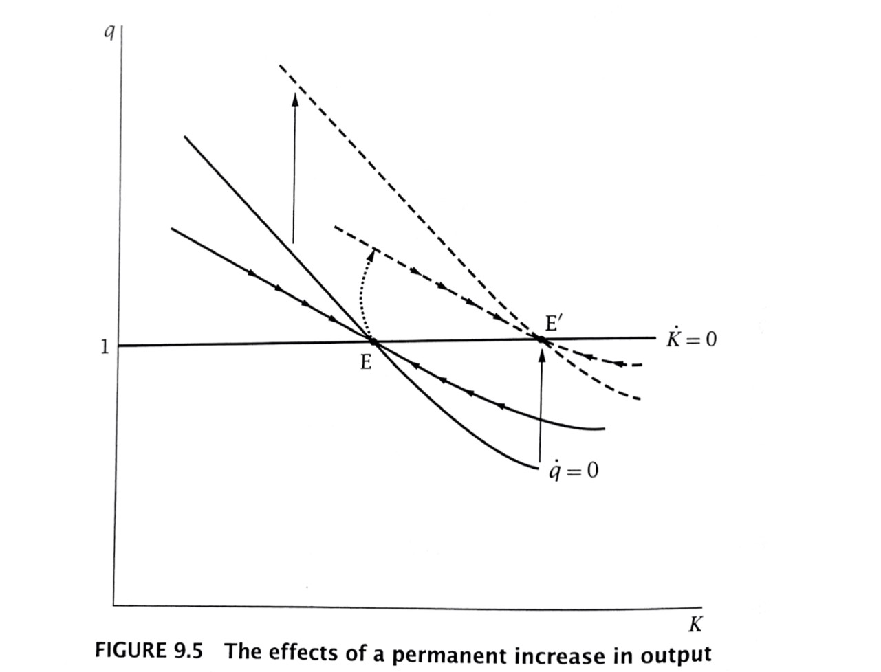
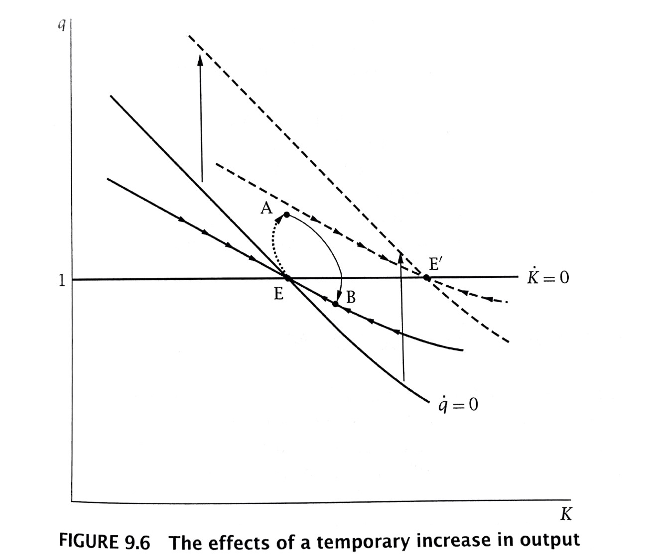
Unit 7.6:The Steady State, Transition Dynamics and Phase Diagrams
We have two dynamic equations:
We represent these dynamic equations diagrammatically
First, note the steady state definition as some $k^,q^$ such that
Exploring the dynamics of capital
For capital,
- And note, for $q>1,\Delta k_t>0$
- For $q<1,\Delta k_t<0$
We can draw this in $\{q,k\}$
Exploring the dynamics of stock prices
For stock prices,
- And note, for $q>\frac{f’(k_t)}{r_t}$, $\Delta q_t>0$
- Since $f’(k_t)$ is declining in $k_t$, it looks like this:
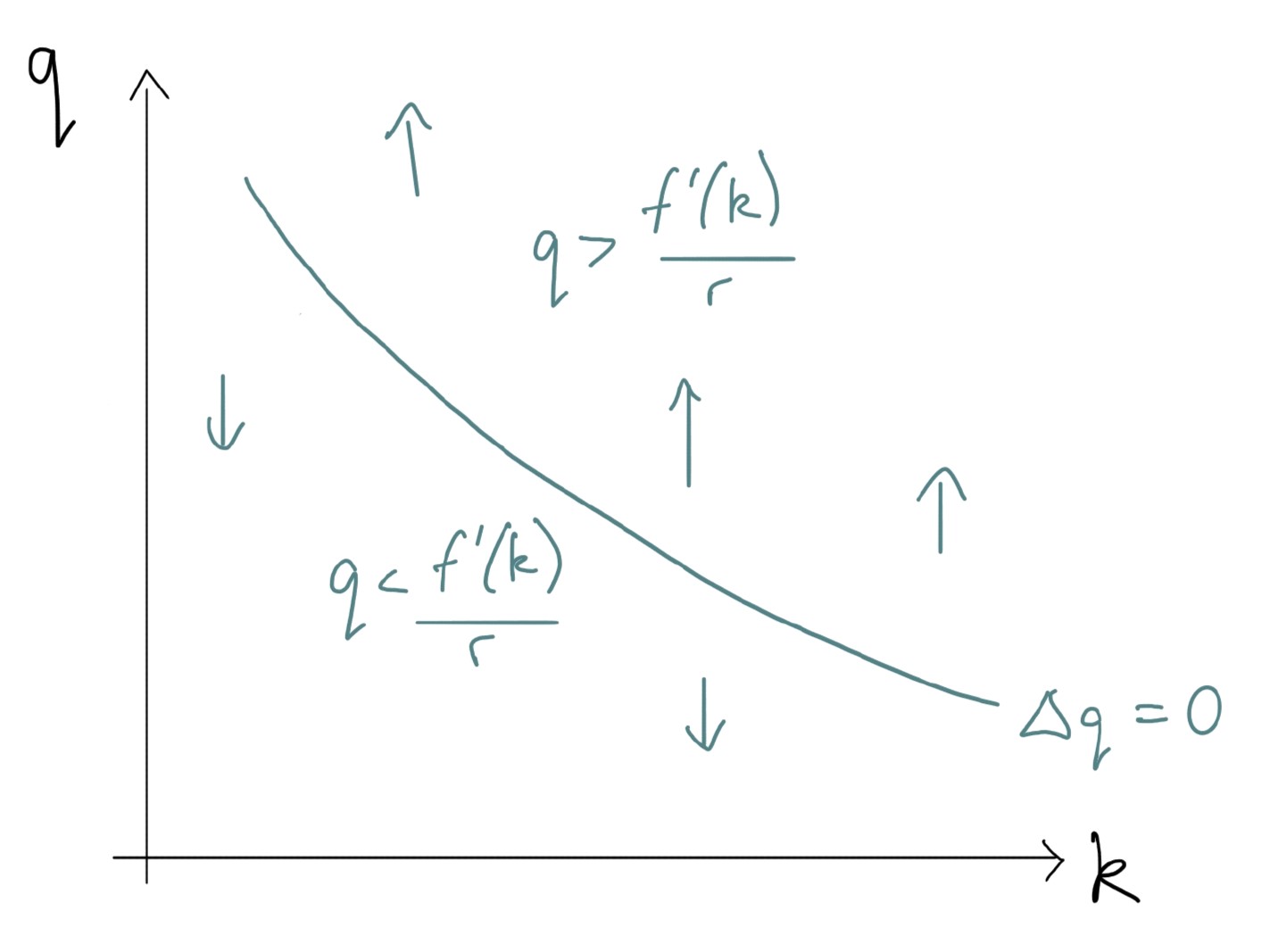
Putting it all together
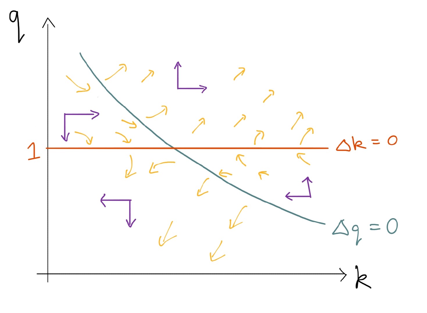
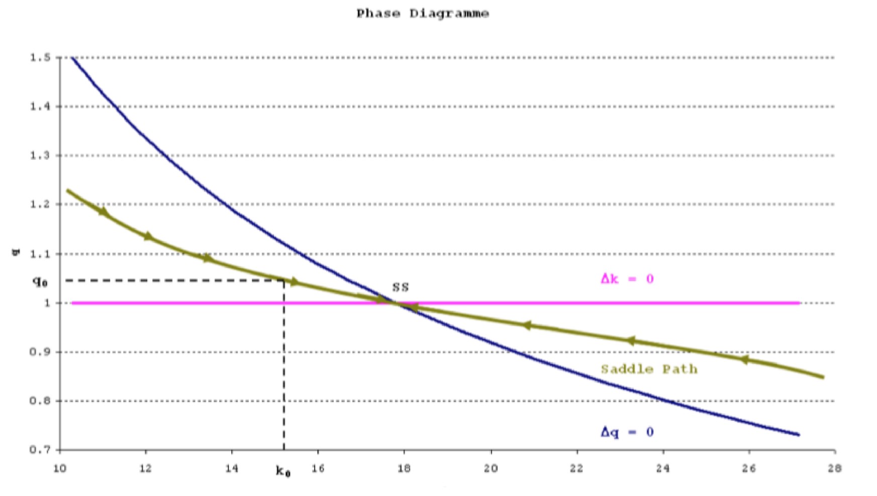
Saddle Path
The Saddle Path is the path along which the dynamical system ends up at the steady state
Thus, for an initial $k_0$, there is an initial $q_0$ on that saddle path
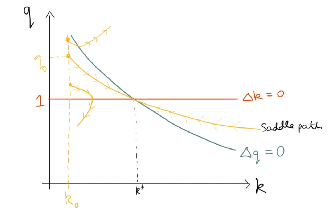
Shocks and government policies
We can use this framework to look at the impact of, e.g., macro shocks on stock prices
- There are lots of examples in Romer
Important note:
- We have a ‘jump’ variable, $q_t$
- And a ‘predetermined’ variable, $k_t$
Thus, in response to some shock, the $q$ jumps onto a new saddle path (if there is one), and the $k$ does not immediately change
Permanent increase in output
Temporary increase in output
Permanent fall in interest rate
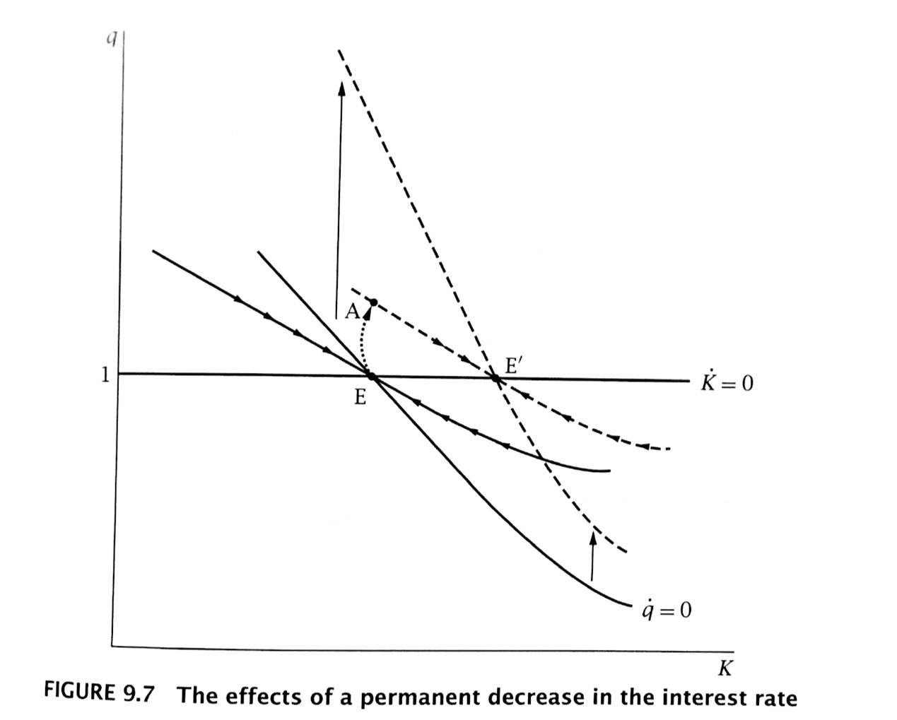
$q\rightarrow \Delta k\rightarrow i\rightarrow q\rightarrow k$
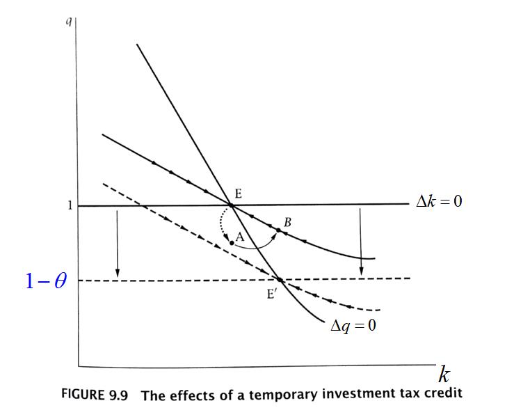
Investment subsidy
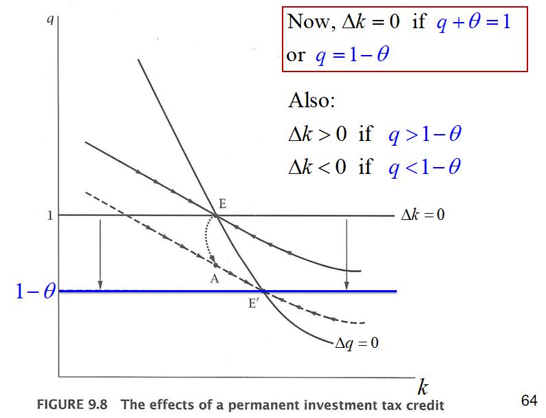
- $\theta$ : tax credit
Temporary tax credit
Topic 7 总结
- tobin’s q
Leased Capital
- regular production function :$f$
own capital, without adjustment costs
- utility of the representative shareholder :$u(c_t)$
- investment :$i$
- consumption of shareholder :$c$
- price of a share :$p$
own capital, with adjustment costs
unit installation cost :$T$
total cost of capital increase :$i_t[1+T(\frac{i_t}{k_t})]$
- debt : $b_0$
- shareholder’s instantaneous utility
- discounts utility rate :$\rho$
- shadow price of installed capital :$q$
If $i_t>0$
If $i_t<0$