【代码】Lab of Applied Computational Finance

基于格拉斯哥ECON5065中Lab的代码的笔记；

如果需要代码与数据可以在本人Github页面上找到

Week 2: Newton’s method to compute implied volatility

此部分对应于笔记中的 Unit 1.5 。首先，我们用牛顿法对 implied volatility 进行估计，然后将结果画成 implied volatility surface，并与 Matlab 自带的求解 implied volatility 的公式 blsimpv 比较。期权数据来自于 Yahoo Finance。

function vol=newtoniv(S,K,r,T,price,callput)
% S is stock price, 
% K is strike price,  
% r is free interest rate, 
% T is time to maturity, 
% price is market option price,
% callput is 1 if call 0 if put

vol     = 1.0; % initial value of implied volatility
sigma   = vol+0.1; % sigma is volatility in BS model
maxiter = 20;
tol     = 1e-4;
iter    = 0;

% newton-raphson method
while abs(sigma-vol)>tol || iter < maxiter % precision of result
    sigma = vol;
    d1    = (log(S/K)+(r+sigma^2/2)*T)/(sigma*sqrt(T));
    d2    = d1-sigma*sqrt(T);
    if callput == 1
        cp = S*normcdf(d1)-K*exp(-r*T)*normcdf(d2);   %European call option price under BS model
    else
        cp = K*exp(-r*T)*normcdf(-d2) - S*normcdf(-d1);   %European put option price under BS model
    end
    vega   = S*sqrt(T)*normpdf(d1);% call/put vega
    fsigma = cp-price;
    vol    = sigma-fsigma/vega;% 期权对 sigma 的偏导即 vega
    iter   = iter + 1;
end

$\sigma_{k+1} = \sigma_k - \frac{C(t,T, \sigma_k,K)-C^{obs}(t)}{\frac{\partial}{\partial \sigma}C(t,T, \sigma_k,K)}$

在验证的过程中，使用 Matlab 公式 blsimpv - Black-Scholes implied volatility

This MATLAB function using a Black-Scholes model computes the implied volatilityof an underlying asset from the market value of European call and put options.
1
>Volatility = blsimpv(Price,Strike,Rate,Time,Value)

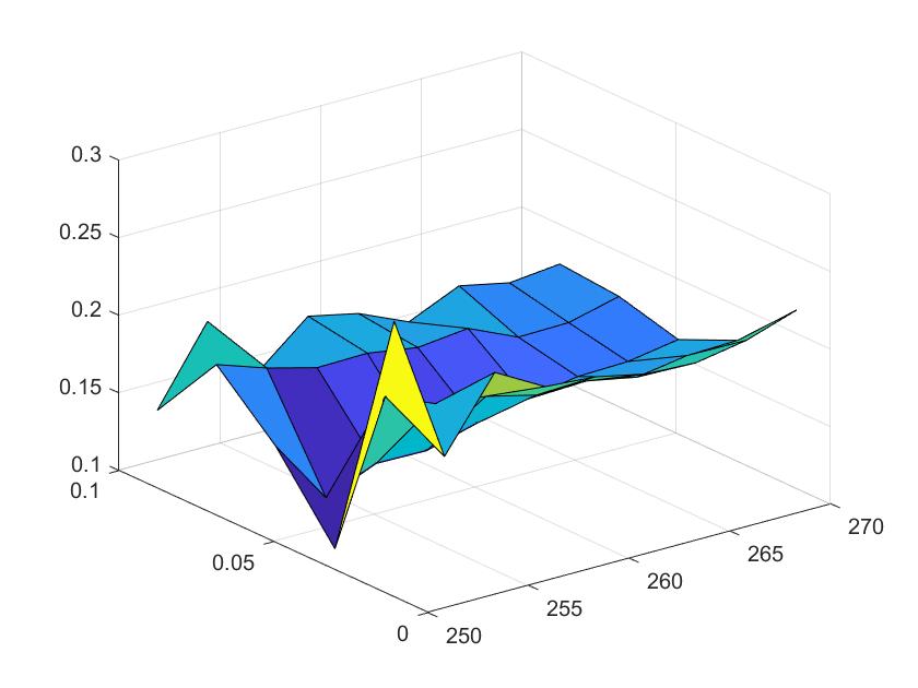
S=260.05;% stock price
r=0.02; % interest rate
T=[4/365,11/365,18/365,25/365,32/365]; % time maturity
K=[250,252.5,255,257.5,260,262.5,265,267.5,270];%strike price
C=[ 10.4 7.73 5.8 3.8 2.3 1.19 0.55 0.25 0.12;
    10.24 8.69 6.6 4.85 3.3 2.2 1.29 0.81 0.46;
    10.9 8.23 6.4 4.65 3.42 2.45 1.72 1.11 0.75;
    12 9.89 7.95 6.4 4.9 3.84 2.52 1.8 1.4;
    11.57 10.83	8.02 7.26 5.7 4.1 3.55 2.54 1.97;];%prices for different maturities in rows
volatility=zeros(5,9);
% plot implied volatility surface
[x,y]=meshgrid(K,T);
for i=1:5  
   for  j=1:9
     volatility(i,j)=blsimpv(S,K(j),r,T(i),C(i,j));
   end
end
surf(x,y,volatility)

for i=1:5  
   for  j=1:9
     volatility(i,j)=newtoniv(S,K(j),r,T(i),C(i,j),1);
   end
end
surf(x,y,volatility)

我们可以发现结果是很相似的

Week 3: Delta-hedging in the Black-Scholes model

此部分主要计算采用 Delta 对冲后的策略价值。首先我们引入股票价格的增长公式

function ST=BSpath(S0,mu,sigma,T,n,N)
% S0 is the initial stock price, 
% K is strike price,  
% r is free interest rate, 
% T is time to maturity, 
% n is the number of time discretisation steps,
% N is the sample size
% mu is the asset's rate of return 
% sigma is the asset's volatility

nstep = power(2,n); % 步数
delt = T/nstep; % 每步时间间隔
const = ones(N,nstep+1)*(mu - 0.5*sigma*sigma)*delt; % 计算 s（t+1）时固定增长量
BMval = normrnd(0,1,[N,nstep+1]); % Brownian Motion Value/Matrix
BMval(1:N,1) = 0;
const(1:N,1) = 0;
incr = const + sigma*sqrt(delt)*BMval;
ST = S0*cumprod(exp(incr));
end

其中 cumprod 输出的是累计乘积的值

cumprod([1 2 3])

ans =
1
1     2     6

因此 BSpath 输出的是股票波动的路径。我们在此基础上建立对冲资产组合的路径。

function [X,PNL]=deltahedge(S0,K,r,mu,sigma,T,n,N)
% S0 is the initial stock price, 
% K is strike price,  
% r is free interest rate, 
% T is time to maturity, 
% n is the number of time discretisation steps,
% N is the sample size
% mu is the asset's rate of return 
% sigma is the asset's volatility

strike = K;
nstep = power(2,n); % number of time steps
delt = T/nstep;% time step size
tstep = linspace(0,T,nstep+1);
const = ones(N,nstep+1)*(mu - 0.5*sigma*sigma)*delt;
BMval = normrnd(0,1,[N,nstep+1]); % Brownian motion increments
BMval(1:N,1) = 0;
const(1:N,1) = 0;
incr = const + sigma*sqrt(delt)*BMval;
ST = S0*cumprod(exp(incr),2);
% Compute delta at each readjustment time
tt = T-tstep(1:nstep); % 剩余时间
X = zeros(N,length(K)); % final value of the self-financing portfolio
PNL = zeros(N,length(K)); % Profit and loss over Monte Carlo sample paths

for i=1:N
    for j=1:length(K)
        price = blsprice(S0,strike(j),r,T,sigma); % Black-Scholes call price
        d1 = (log(ST(i,1:nstep)./(strike(j)*exp(-r*tt))) + 0.5*sigma*sigma*tt)./(sigma*sqrt(tt));
        delta = normcdf(d1); % 每时期对冲需要的股票数
        temp = ST(i,2:nstep+1).*exp(-r*tstep(2:nstep+1)) - ST(i,1:nstep).*exp(-r*tstep(1:nstep)); % 每时期持有一单位股票收益
        chng = delta.*temp;
        X(i,j) = exp(r*T)*(price +sum(chng));
        PNL(i,j) = exp(-r*T)*(X(i,j) - max(ST(i,nstep+1)-strike(j),0));
    end
end
end

S0 = 100; %Starting price
r = 0.05; %interest rate
T = 1; %call option maturity
n = 5; %exponent in the number of time steps
N = 1000; %number of Monte Carlo sample paths
mu = 0.02; %asset return
sigma = 0.2; %volatility parameter
K = 80; %option strike

[X,PNL]=deltahedge(S0,K,r,mu,sigma,T,n,N);
mean(PNL)
var(PNL)

如果将 n 从 5 增长到 8/10。Mean 和 Var 将由下表所示

n =	5	8	10
Mean	0.01219	0.00385	0.00122
Var	0.31075	0.04385	0.01038

从中我们可以发现，收益的均值随着对冲的频率增加而减少，但是波动也随之减少。另外，虽然我们的结果显示收益大多为正数，但是在我们的代码中并没考虑到交易成本这一问题，在现实的交易中，频繁的交易可能会带来大量的手续费。因此，在动态对冲中，过于频繁地调整组合也不一定是一件好事。

Week 4: Pricing European options in Heston‘s model using inverse Fourier transform

此部分对应于笔记中的 Unit 2.9 。普通定价模型中将风险定义为一个常量，而Heston’s Stochastic Volatility Model 则将其定义为一个随时间变换的值。并且 sigma 的值是 mean-reversion 的。如果它偏离了 mean 会有一种力量把它纠正回原点的方向。

$\frac{dS_t}{S_t}=rdt+\sigma_tdW_t$ $\begin{align} &d\sigma_t^2=k(\theta-\sigma_t^2)dt+\delta\sigma_tdW'_t,\ d\langle W,W'\rangle_t=\rho dt\\ or,\ &dv_t=k(\theta-v_t)dt+\delta\sqrt{v_t}dW'_t,\ with\ v_t=\sigma_t^2 \end{align}$

解出定价公式需要用到 Fourier transform 的知识，但这在我们的课程中并不做要求。

function call = HestonCallQuad(kappa,theta,sigma,rho,v0,r,T,s0,K)
warning off;
call = s0*HestonP(kappa,theta,sigma,rho,v0,r,T,s0,K,1) - ...
K*exp(-r*T)*HestonP(kappa,theta,sigma,rho,v0,r,T,s0,K,2);

function ret = HestonP(kappa,theta,sigma,rho,v0,r,T,s0,K,type)
ret = 0.5 + 1/pi*quadl(@HestonPIntegrand,0,100,[],[],kappa, ...
theta,sigma,rho,v0,r,T,s0,K,type);

function ret = HestonPIntegrand(phi,kappa,theta,sigma,rho, ...
v0,r,T,s0,K,type)
ret = real(exp(-1i*phi*log(K)).*Hestf(phi,kappa,theta,sigma, ...
rho,v0,r,T,s0,type)./(1i*phi));

function f = Hestf(phi,kappa,theta,sigma,rho,v0,r,T,s0,type)
if type == 1
u = 0.5;
b = kappa - rho*sigma;
else
u = -0.5;
b = kappa;
end
a = kappa*theta; x = log(s0);
d = sqrt((rho*sigma*phi.*1i-b).^2-sigma^2*(2*u*phi.*1i-phi.^2));
g = (b-rho*sigma*phi*1i + d)./(b-rho*sigma*phi*1i - d);
C = r*phi.*1i*T + a/sigma^2.*((b- rho*sigma*phi*1i + d)*T - ...
2*log((1-g.*exp(d*T))./(1-g)));
D = (b-rho*sigma*phi*1i + d)./sigma^2.*((1-exp(d*T))./ ...
(1-g.*exp(d*T)));
f = exp(C + D*v0 + 1i*phi*x);

Matlab 强大的数学运算功能提供了我们一个非常方便的工具来运算解，使用 quadl 来进行数值积分大大减少了我们的负担。但值得注意的是，quadl 进行的运算是以矩阵的形式，因此进行积分的公式需要兼容矩阵运算的格式。

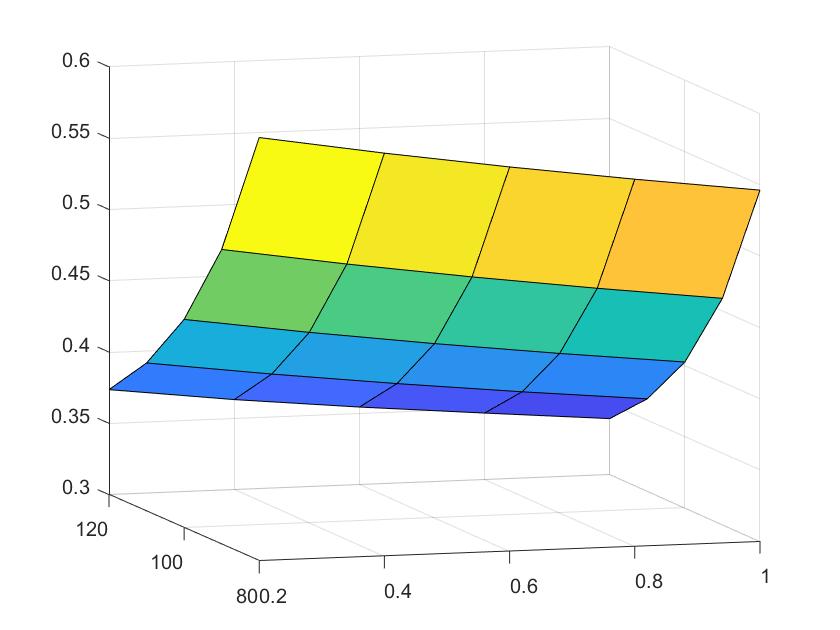
% initialization of parameters for Heston model
s0=100;% stock price
r=0.02; % interest rate
kappa=5; % speed of mean reversion
theta=0.04;% long term mean
sigma=0.5; % volatility of volatility
rho=-0.7;
v0=0.5;% initial variance
T=[0.2,0.4,0.6,0.8,1]; % time maturity
K=[80,90,100,110,120]; % strike price

C=zeros(5,5);
for i=1:5
    for j=1:5
        C(i,j)=HestonCallQuad(kappa,theta,sigma,rho,v0,r,T(i),s0,K(j)); % European call option price under Heston model
    end
end

volatility=zeros(5,5);
% plot implied volatility surface
[x,y]=meshgrid(T,K);
for i=1:5
   for  j=1:5
     volatility(i,j)=blsimpv(s0,K(j),r,T(i),C(i,j));
   end
end
surf(x,y,volatility)

如果将 sigma=0.5 代入 Heston’s Model 求出的值重新用 blsimpv 求 volatility。我们可以从图中发现，结果确实是围绕在 0.5 附近的。

Week 5: Calibration of Heston’s model to market data

但实际上 Heston’s model 的准确度非常依赖它的系数与波动率初始值（$\kappa,\theta,\sigma,\rho,v_0$）。因此，在运用模型之前还需要运用 lsqnonlin 对模型的系数进行训练。如果令 $\Theta = (\kappa,\theta,\sigma,\rho,v_0)$，优化函数则是

$\min_{\Theta}\sum_{i,j}w_{i,j}(P^{model(\Theta)}(T_i,K_j)-P^{market}(T_i,k_j))^2$ $w_{ij}=\frac1{|P^{market,bid}(T_i,K_j)-P^{market,ask}(T_i,K_j)|}$ $P^{market}(T_i,k_j)=\frac{P^{market,bid}(T_i,K_j)+P^{market,ask}(T_i,K_j)}2$

function ret = HestonDifferences(input)
global NoOfOptions;
global OptionData;
global NoOfIterations;
global PriceDifference;
NoOfIterations = NoOfIterations + 1;
%counts the no of iterations run to calibrate model
for i = 1:NoOfOptions
PriceDifference(i) = (OptionData(i,5)-HestonCallQuad( ...
(input(1)+input(3)^2)/(2*input(2)),input(2),input(3),input(4),input(5), ...
OptionData(i,1),OptionData(i,2),OptionData(i,3),OptionData(i,4)))...
/sqrt((abs(OptionData(i,6)- OptionData(i,7))));
%Option Value-Estimated Value(4个系数，4个已知)
%kappa=(?+sigma^2)/2theta,theta,sigma,rho,v0,r,T,s0,K
%sqrt((abs(OptionData(i,6)-OptionData(i,7))))-> w_ij (weight)
end
ret = PriceDifference';

因为要求 $\kappa > \sigma^2/2\theta$ ，input(1) 需要大于0

clear;
global OptionData;
global NoOfOptions;
global NoOfIterations;
global PriceDifference;
NoOfIterations = 0;
load OptionData.m ;
%OptionData = [r,T,S0,K,Option Value,bid,offer]
Size = size(OptionData);
NoOfOptions = Size(1);
%input sequence in initial vectors [2*kappa*theta - sigma^2,theta,sigma,rho,v0]
%x0 = [0.05 0.05 0.5 -0.5 0.15];
x0 = [0.5 0.1 1.3 -0.75 0.2]; % 系数训练初始值
lb = [0 0 0 -1 0]; % 系数训练最小值
ub = [20 1 5 0 1]; % 系数训练最大值
options = optimset('MaxFunEvals',20000);
%sets the max no. of iteration to 20000 so that termination doesn't take place early.
tic;
Calibration = lsqnonlin(@HestonDifferences,x0,lb,ub);
toc;
Solution = [(Calibration(1)+Calibration(3)^2)/(2*Calibration(2)), Calibration(2:5)];
%output sequence in Solution = [kappa,theta,sigma,rho,v0]

Week 6: Pricing of European option in Heston’s model using the Monte Carlo method

此部分对应于笔记中的 Unit 3.1 。蒙特卡洛部分要使用 Euler-Maruyama 和 Milstein schemes 两种方法来运算，并且对比。

% European call option under Heston model with Euler-Maruyama-Method and Milstein method
clear all;
M = 50000; % number of paths
N = 100;% number of time steps
T = 1;% maturity
h = T/N;%delta t
S0 = 100; 
sigma20 = 0.0625; %variance at t=0
K=100; % strike
kappa = 2;
theta = 0.4;
nu = 0.2;
rho = -0.7;
r=0.02;

% two dimensional Brownian motion
dW1 = randn(M,N+1)*sqrt(h);
dW2 = rho*dW1 + sqrt(1-rho^2)*randn(M,N+1)*sqrt(h);

Euler Maruyama method 的主要公式是

$dX(t)=b(t,X(t))dt+\sigma(t,X(t))dW_t$ $X_n^h:=X(t_n^h)=X_{n-1}^h+b(t_{n-1}^h,X_{n-1}^h)h+\sigma(t_{n-1}^h,X_{n-1}^h)\Delta W_n^h$

其中

$b(t,X(t))\Rightarrow k(\theta-\sigma_t^2)dt\quad \sigma(t,X(t))\Rightarrow\delta\sigma_tdW'_t$

% Initialisation of stock price and volatility for Euler Maruyama method
S = S0*ones(M,N+1);
sigma2 = sigma20*ones(M,N+1);

% Solution of the SDE-System with Euler-Maruyama-Method
% NOTE: we don't need to store the entire simulation path to compute the 
%European option payoff!
for i = 1:N
    sigma2(:,i+1) = sigma2(:,i) + kappa*(theta-sigma2(:,i))*h ...
        + nu*sqrt(abs(sigma2(:,i))).*dW2(:,i);
    S(:,i+1) = S(:,i).*(1 + r*h + sqrt(abs(sigma2(:,i))).*dW1(:,i));
end

payoff = exp(-r*T)*max(0,S(:,end)-K);
stdpayoff = std(payoff);
V = mean(payoff)
Vleft = V - 1.96*stdpayoff/sqrt(M)
Vright = V + 1.96*stdpayoff/sqrt(M)

Milstein Scheme 的主要公式是

$X_n^h=X(t_n^h)=X_{n-1}^h+bh+\sigma\Delta W_n^h+\frac12\partial_x\sigma\sigma_t((\Delta W_n^h)^2-h)$

其中

$\partial_x\sigma\Rightarrow \partial_{\sigma^2}\delta\sigma_t=\frac\delta{2\sigma_t}$

% Initialisation of stock price and volatility for Milstein method
S1 = S0*ones(M,N+1);
sigma3 = sigma20*ones(M,N+1);
% Solution of the Milstein method

for i = 1:N
    sigma3(:,i+1) = sigma3(:,i) + kappa*(theta-sigma3(:,i))*h ...
        + nu*sqrt(abs(sigma3(:,i))).*dW2(:,i)+1/4*nu.*(dW2(:,i).^2-h);
    S1(:,i+1) = S1(:,i).*(1 + r*h + sqrt(abs(sigma3(:,i))).*dW1(:,i))+1/2*sigma3(:,i).*S1(:,i).*(dW1(:,i).^2-h);
end

payoff1 = exp(-r*T)*max(0,S1(:,end)-K);
stdpayoff1 = std(payoff1);
V1 = mean(payoff1)
V1left = V1 - 1.96*stdpayoff1/sqrt(M)
V1right = V1 + 1.96*stdpayoff1/sqrt(M)

运算的结果，可以与前面的 HestonCallQuad 进行确认

Week 7: Variance reduction method in the Black-Scholes model for Asian option pricing

此部分对应笔记中的 Unit 3.2.1。我们想要预测 Arithmetic average Asian call option 的价格，同时将 Geometric average Asian option 作为 control variate 来降低预测值的 VAR。在代码中使用的 Geometric Asian option 的定价方程参考于 Nielsen 的论文《Pricing Asian Options》^[1]^。

function [Pasian_cv,CIasian_cv,Pasian,CIasian,Pgm,CIgm,Pgeo] = asiancall_cv(S0,K,r,sigma,T,n,N,b)
dt= T/n;
R = exp(-r*T);
m = (r - sigma^2/2)*dt;
s = sigma*sqrt(dt);
Vcall = zeros(1,N);
Vgmcall = zeros(1,N);
for j = 1:N
    Z= m+s*randn(1,n);
    S = cumsum([log(S0), Z],2);
    Vcall(j) = max(mean(exp(S))-K,0); % Arithmetic average
    Vgmcall(j) = max(exp(mean(S))-K,0); % Geometric average
end
Pasian = mean(R*Vcall); 
CIasian = std(R*Vcall)/sqrt(N);
Pgm = mean(R*Vgmcall);
CIgm = std(R*Vgmcall)/sqrt(N);

sigmaG = sigma*sqrt(dt*(2*n+1)*(n+1)/(6*n));
muG = log(S0) + 1/2*(r-sigma^2/2)*(T+dt);
d1 = (muG -log(K) + sigmaG^2)/sigmaG;
d2 = d1 - sigmaG;
Pgeo = R*(exp(muG+0.5*sigmaG^2)*normcdf(d1) - K*normcdf(d2)); % the price of Geometric Asian option

Pasian_cv = R*Vcall - b*(R*Vgmcall-Pgeo);
CIasian_cv = std(Pasian_cv)/sqrt(N);
Pasian_cv = mean(Pasian_cv);

Variance reduction 主要的部分是

$Y_i(\hat b_N):=Y_i-\hat b_N(X_i-\alpha_0)$

$\alpha_0$ ：Pgeo
变量 $\hat b_N$ 的值是一个固定的数，需要预先拟合出来。

$b^*=\frac{Cov(X,Y)}{Var(X)}$

[1] Nielsen, L. Pricing Asian Options. Master of Science Dissertation, University of Aarhus

Week 8: Finite difference method to solve the Black-Scholes PDE

此部分对应笔记中的 Unit 4.1 。代码只包括 Explicit Scheme 的部分，对于 Implicit Scheme 的部分需要用到 c 语言编写的程序 thomas，暂时没有进行详细的阅读，就不放在笔记中了。更多相关知识也可以搜索数值分析课程进行学习。

clear all
close all

J=1000;
S0=17;
% time steps to ensure numerical convergence
N = J^2;
K = 15;
logstrk = log(K);
T=0.3041;
r=0.03;
sigma = 0.25;
mu = r - 0.5*sigma^2;
xmin = log(10e-6);
xmax = log(2*K);
dx=(xmax-xmin)/J; 
x=[xmin:dx:xmax]'; %length = J+1
dt=T/N;

V=max(0,exp(x)-K);
Vold=V;
const1 = 1 - sigma^2*dt/dx^2;
const2 = 0.5*sigma^2*dt/dx^2;
const3 = 0.5*mu*dt/dx;

for n=1:N 
    %boundary condition at x = xmin  
    V(1)=0;  
        
    for j=2:J %in the interior
        V(j)= Vold(j)*const1 + Vold(j+1)*(const2+const3) + Vold(j-1)*(const2-const3) - r*dt*Vold(j);
    end
    
    %boundary condition at x = xmax
    V(J+1)= exp(xmax)-K;
    
    Vold=V;
end

V_Final = interp1(x, V, log(S0));

figure(1)
clf
plot(exp(x),V)
xlabel('asset price')
ylabel('call price')

Week 9: Finite difference method to solve the Heston model PDE

本章代码是根据 Sensen Lin 的论文《Finite Difference Schemes for Heston Model》^[2]^。其中定义 Heston model

$d S=\mu S d t+\sqrt{v(t)} S d z_{1}(t)$ $d v(t)=\kappa[\theta-v(t)] d t+\delta\sqrt{v(t)} d z_{2}(t)$

那么期权合约 C 服从 partial differential equation

$\begin{align} \frac{1}{2} v S^{2} \frac{\partial^{2} C}{\partial S^{2}}+\rho \delta v S \frac{\partial^{2} C}{\partial S \partial v}+\frac{1}{2} \delta^{2} v \frac{\partial^{2} C}{\partial v^{2}}+r S \frac{\partial C}{\partial S} \\ +\kappa(\theta-v(t))\frac{\partial C}{\partial v}-r C+\frac{\partial C}{\partial t} & = 0 \end{align}$

其边界条件为

$\begin{align} &C(s, v, T) = \max (0, s-K) \\ &C(0, v, T) = 0 \\ &C(s, \infty, t) = s\\ &\frac{\partial C}{\partial s}(\infty, v, t) = 1 \\ &r s \frac{\partial C}{\partial s}(s, 0, t)+\kappa \theta\frac{\partial C}{\partial v}(s, 0, t)-r C(s, 0, t)+\frac{\partial C}{\partial t}(s, 0, t) = 0 \end{align}$

公式中的偏导部分可以变换为

$\begin{align} &\frac{\partial C}{\partial S}(i\Delta s,j\Delta v) \approx \frac{C_{i+1, j}-C_{i-1, j}}{2 \Delta s} \\ &\frac{\partial C}{\partial v}(i\Delta s,j\Delta v) \approx \frac{C_{i, j+1}-C_{i, j-1}}{2 \Delta v} \\ &\frac{\partial^{2} C}{\partial S^{2}}(i\Delta s,j\Delta v) \approx \frac{C_{i+1, j}-2 C_{i, j}+C_{i-1, j}}{(\Delta s)^{2}} \\ &\frac{\partial^{2} C}{\partial v^{2}}(i\Delta s,j\Delta v) \approx \frac{C_{i, j+1}-2 C_{i, j}+C_{i, j-1}}{(\Delta v)^{2}} \\ &\frac{\partial^{2} C}{\partial S \partial v}(i\Delta s,j\Delta v) \approx \frac{C_{i+1, j+1}+C_{i-1, j-1}-C_{i-1, j+1}-C_{i+1, j-1}}{4 \Delta s \Delta v} \end{align}$

代入原式则变换为

$\begin{align} &\frac{c_{i, j}^{n+1}-c_{i, j}^{n}}{\Delta t} = \left[\left(s_{i}\right)^{2} v_{j} \frac{c_{i+1, j}-2 c_{i, j}+c_{i-1, j}}{2(\Delta s)^{2}}+\rho \delta s_{i} v_{j} \frac{c_{i+1, j+1}+c_{i-1, j-1}-c_{i-1, j+1}-c_{i+1, j-1}}{4 \Delta s \Delta v}\right. \\ &\left.+\delta^{2} v_{j} \frac{c_{i, j+1}-2 c_{i, j}+c_{i, j-1}}{2(\Delta v)^{2}}+r s_{i} \frac{c_{i+1, j}-c_{i-1, j}}{2 \Delta s}+\kappa\left(\theta-v_{j}\right) \frac{c_{i, j+1}-c_{i, j-1}}{2 \Delta v}-r c_{i, j}\right]^{n} \end{align}$

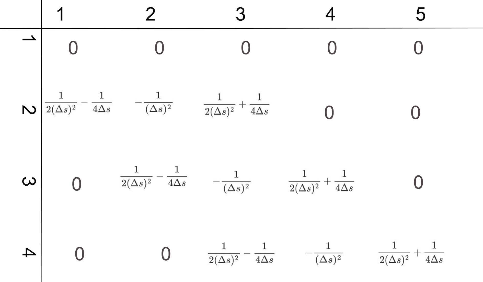
function Un=hestonPDEprice(kappa,theta,delta,rho,T,dt,K,Y,I,J)
    %hestonPDEprice(1.15,0.10,0.2,-0.4,4/52,4/(52*4000),40,1.0,80,40)
    nt=ceil(T/dt);
    xmin = log(1e-2);
	xmax = log(2.0*K);
    ymin = 0;
    ymax = Y*1.2;
    dx = (xmax-xmin)/I; %step length of x
    dx2 = dx*dx;
    dy = Y/J; %step length of y
    dy2 = dy*dy;
    xvalue = xmin:dx:xmax; %grid of x values
    yvalue = ymin:dy:ymax; %grid of y values
    nx = length(xvalue)-1; %number of entries in x axis - 1
    ny = length(yvalue)-1; %number of entries in y axis - 1
    temp = max(exp(xvalue)-K,0); %European call payoff: terminal condition
    uinitial = temp'*ones(1,ny+1); %x in row i, vol in col j
    U = uinitial; % u in dimension of (nx+1)*(ny+1)
    for n=1:nt
        %interior elements in cross derivative
        Upp = U(3:nx+1,3:ny+1); %+1 in x, +1 in y
        Umm = U(1:nx-1,1:ny-1); %-1 in x, -1 in y
        Ump = U(1:nx-1,3:ny+1); %-1 in x, +1 in y
        Upm = U(3:nx+1,1:ny-1); %+1 in x, -1 in y
        Uxy = Upp+Umm-Ump-Upm;
        G0t = (rho*delta*dt/(4*dx*dy))*ones(1,nx+1)'*yvalue;
        G0 = G0t(2:nx,2:ny);        
        U1t = G0.*Uxy;
        U1 = [zeros(1,ny+1);zeros(nx-1,1) U1t zeros(nx-1,1);zeros(1,ny+1)];% pad with zeros at the edge of domain
        % dsdv 项以及其前面的系数
        
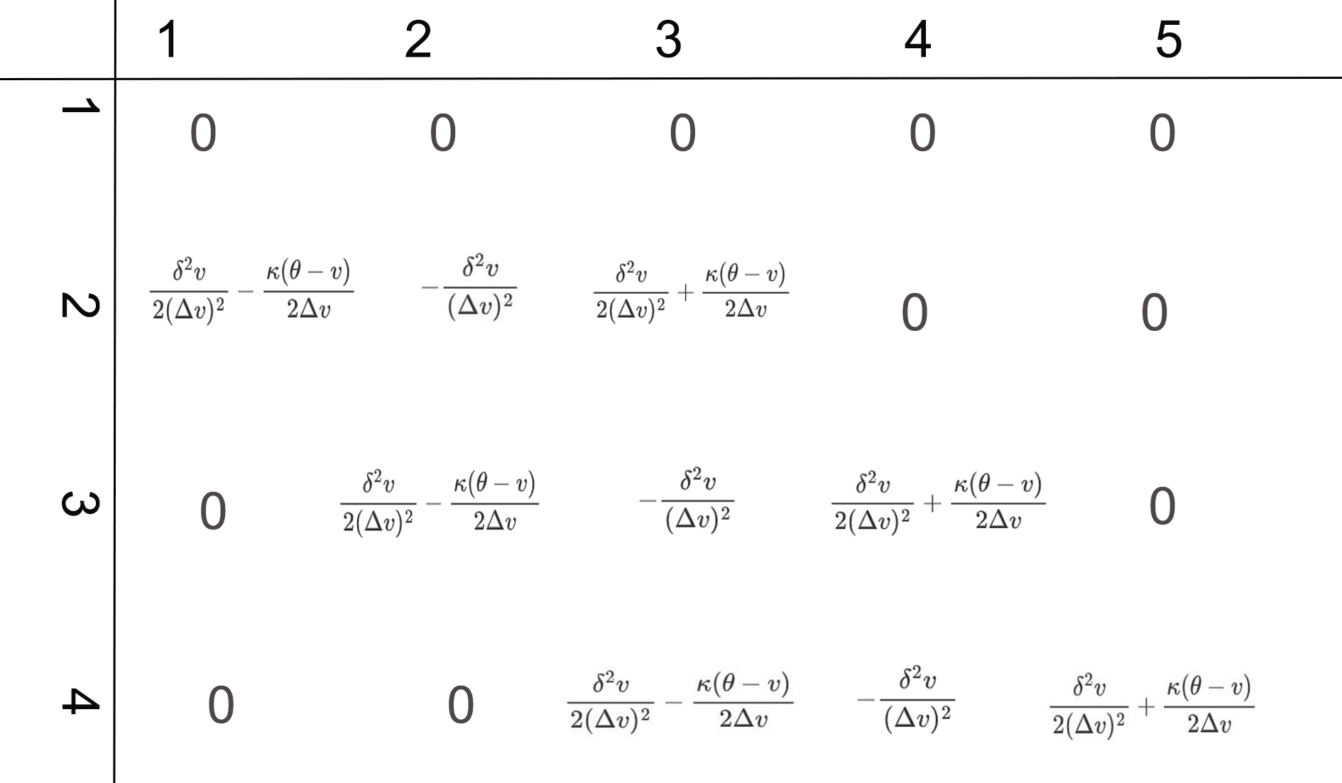
        % elements in X direction
        C1 = ones(1,nx-1)*(0.5/dx2 + 0.25/dx);
        C1 = [C1';0;0];
        A1 = -ones(1,nx-1)/dx2; 
        A1 = [0;A1';0];
        E1 = ones(1,nx-1)*(0.5/dx2 - 0.25/dx);
        E1 = [0;0;E1'];
        %sparse matrix with A1 on the diagonal, C1 one below & D1 one above
        B = spdiags([C1 A1 E1],[-1 0 1],nx+1,nx+1); 
        for j=2:ny
            A = U(:,j);
            G1 = dt*yvalue(j)*B;
            U2t = G1*A; % the interior elements along the j-th sub-vector.
            U2t(nx+1) = 0; 
            U2t(1) = 0;
            if j==2
                U2 = U2t;
            else
                U2 = [U2 U2t]; % arrange in columns
                % ds,(ds)^2项以及前面的系数
            end
        end
        U2 = [zeros(nx+1,1) U2 zeros(nx+1,1)]; %pad with zeros in the first and last columns
        %
        % elements in Y direction
        E1 = 0.5*delta^2*yvalue(2:ny)/dy2 - 0.5*kappa*(theta-yvalue(2:ny))/dy;
        E1 = [E1';0;0];
        A1 = -delta^2*yvalue(2:ny)/dy2;
        A1 = [0;A1';0];
        F1 = 0.5*delta^2*yvalue(2:ny)/dy2 + 0.5*kappa*(theta-yvalue(2:ny))/dy;
        F1 = [0;0;F1'];
        D = spdiags([E1 A1 F1],[-1 0 1],ny+1,ny+1);
        for i = 2:nx
            A = U(i,:)';
            U3t = dt*D*A;
            U3t(1) = 0;
            U3t(ny+1) = 0;
            if i==2
                U3 = U3t';
            else
                U3 = [U3; U3t'];
            end
        end
        U3 = [zeros(1,ny+1);U3;zeros(1,ny+1)];
        % dv,(dv)^2项以及前面的系数
        Uy = U(:,1); % the first column of the previous U
        U = U + U1 + U2 + U3 ;
        % 代入边界条件
        U(1,:) = zeros(1, ny+1); %when x = xmin
        U(:,ny+1) = exp(xvalue)'; %when y = ymax
        % elements where y=0
        for i=2:nx
            U(i,1)=(Uy(i)+kappa*theta*dt*U(i,2)/dy)/(1+kappa*theta*dt/dy);
        end
        U(nx+1,2:ny) = exp(xvalue(nx+1))- K;%when x = xmax
        %U(nx+1,2:ny) = (2*dx*exp(xvalue(nx+1))+4*U(nx,2:ny)-U(nx-1,2:ny))/3;
    end
    Un = U(1:I+1,1:J+1);
    
%     p0 = zeros(nx+1,ny+1);    
%     for i=1:nx+1
%         for j=1:ny+1            
%             p0(i,j) = HestonCallQuad(kappa,theta,delta,rho,yvalue(j),0,T,exp(xvalue(i)),K);
%         end
%     end
%     p = p0(1:I+1,1:J+1);
end

以上代码是以 log(S) 为纵轴方向指标变换的，因此与文章中的代码有些不同。

其中矩阵 B 的样式为

矩阵 D 的样式为

[2] Lin, S. (2008). Finite Difference Schemes for Heston Model. Master of Mathematical and Computational Finance Dissertation, University of Oxford

Week 10: Calibration of Dupire’s model to market data

此部分对应笔记中的 Unit 2 。主要运用两种方法来预测local volatility。第一种是Dupire’s model 的原始公式，公式中参考的是 $q=0$ 的格式

$\sigma^2(T,K)=2\frac{C_T(T,K)+rKC_K(T,K)}{K^2C_{KK}(T,K)}$

第二种方法是 Dupire’s model 的变换形式，其中 $I(T,K)$ 是从 Black-Scholes 中逆向推导过来的 implied volatilities。

$\sigma^2(T,K)=\frac{\frac IT+2I_T+2rKI_K}{K^2(\frac1{K^2IT}+2\frac{d_+}{KI\sqrt{T}}I_K+\frac{d_+d_-}{I}I_K^2+I_{KK})}$

如果运用第一种方法，需要使用大量数据进行偏导取值的趋近计算

%In the data provided, there are non-zero call option prices for 0 maturity.
%In order to do the calculations, drop the values corresponding to 0 maturity. 
T = 0.9;
n = 8;
num_step = 2^n;
S0 = 100;
r = 0.0;
dt = T/num_step;
dK = 0.1;
MaxCounter = 100; %number of maximum iterations for implied vol inversion
MaxVolLevel = 6.0;
N = 1000; %number of Monte Carlo sample paths
        
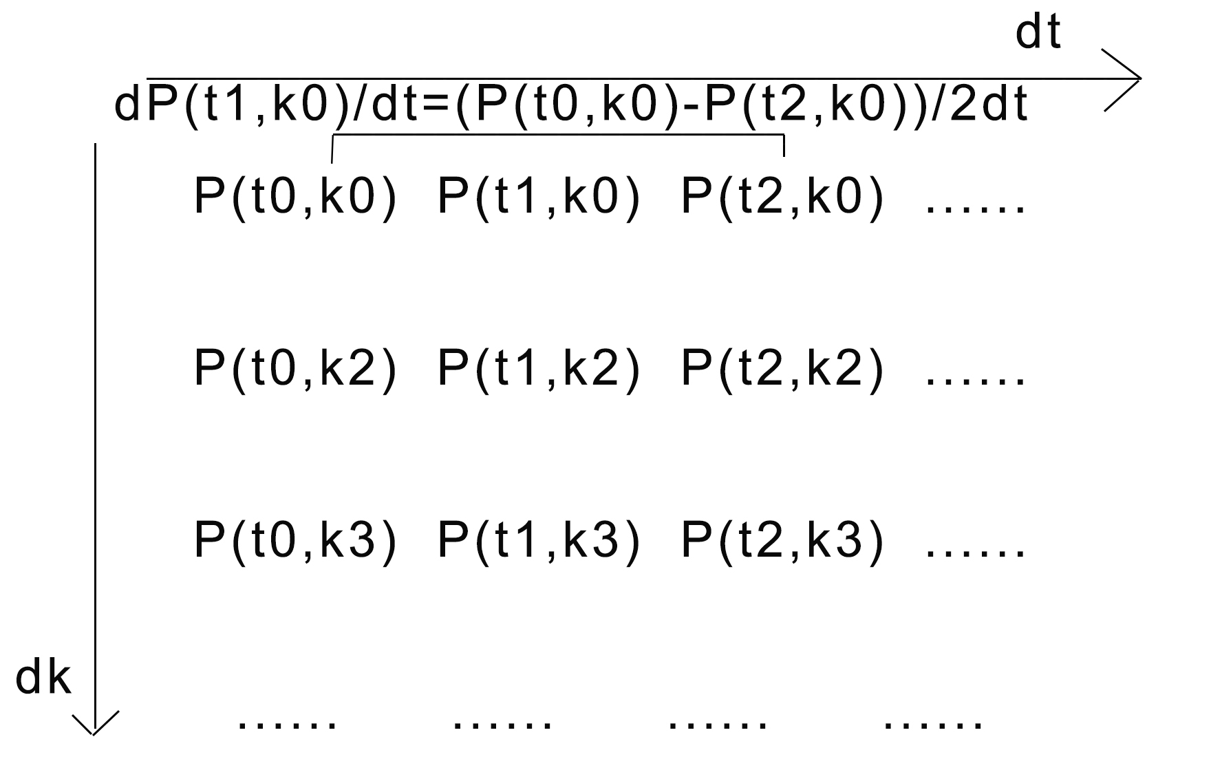
strk = load('strikes.txt'); %strike vector length 401
mat = load('maturities.txt'); %maturity vector length 257
mat = mat(2:end); %remove the maturity 0 entry
pr = load('optionprices.txt'); %price is STRK * MAT 
pr = pr(:,2:end);%remove the prices corresponding to maturity 0
%     
pr_T = zeros(size(pr));
pr_T(1:end,2:end-1) = (pr(1:end,3:end)-pr(1:end,1:end-2))/(2*dt);
pr_T(1:end,1) = (pr(1:end,2)-pr(1:end,1))/dt;
pr_T(1:end,end) = (pr(1:end,end)-pr(1:end,end-1))/dt;
%
pr_K = zeros(size(pr));
pr_K(2:end-1,1:end) = (pr(3:end,1:end)-pr(1:end-2,1:end))/(2*dK);
pr_K(1,1:end) = (pr(2,1:end)-pr(1,1:end))/dK;
pr_K(end,1:end) = (pr(end,1:end)-pr(end-1,1:end))/dK;

pr_KK = zeros(size(pr));
pr_KK(2:end-1,1:end) = (pr_K(3:end,1:end)-pr_K(1:end-2,1:end))/(2*dK);
pr_KK(1,1:end) = (pr_K(2,1:end)-pr_K(1,1:end))/dK;
pr_KK(end,1:end) = (pr_K(end,1:end)-pr_K(end-1,1:end))/dK;

volsq1 = 2.0*(pr_T./(strk.^2.*pr_KK)); %Vol estimate from Dupire formula

进行第二种方法的计算需要先求得 implied volatilities

function callprice = CallBS(S0,K,vol,T,r) %Black-Scholes call price formula
matlen = length(T);
callprice = zeros(size(vol));
for i = 1:matlen
    d1 = (log(S0./K) + (r+0.5*vol(1:end,i).^2)*T(i))./(vol(1:end,i)*T(i)^0.5);
    d2 = d1 - vol(1:end,i)*T(i)^0.5;
    callprice(1:end,i) = S0*normcdf(d1)-K*exp(-r*T(i)).*normcdf(d2);
end

function impvol =  ImpVol(Price,Strike,Maturity,S0,r,MaxIter,MaxVolLevel) %function to find implied vol

volmin = zeros(size(Price));
volmax = MaxVolLevel*ones(size(Price));
vol = 0.5*MaxVolLevel*ones(size(Price));
counter = 0;
while counter < MaxIter % 由二分法进行运算
    CBSImp = CallBS(S0,Strike,vol,Maturity,r);
    temp1 = (CBSImp<=Price);
    temp2 = (CBSImp>Price);
    volmin = temp1.* vol + temp2.*volmin;
    volmax =  (CBSImp<Price).* volmax + (CBSImp>=Price).* vol;
    vol = (volmin + volmax)/2.0;
    counter = counter + 1;
end
impvol = vol;

1	`ivol = ImpVol(pr,strk,mat,S0,0,MaxCounter,MaxVolLevel);`

我们采用相同的方法来对 implied volatilities 的偏导进行运算。

ivol_T = zeros(size(ivol));
ivol_T(1:end,2:end-1) = (ivol(1:end,3:end)-ivol(1:end,1:end-2))/(2*dt);
ivol_T(1:end,1) = (ivol(1:end,2)-ivol(1:end,1))/dt;
ivol_T(1:end,end) = (ivol(1:end,end)-ivol(1:end,end-1))/dt;

ivol_K = zeros(size(ivol));
ivol_K(2:end-1,1:end) = (ivol(3:end,1:end)-ivol(1:end-2,1:end))/(2*dK);
ivol_K(1,1:end) = (ivol(2,1:end)-ivol(1,1:end))/dK;
ivol_K(end,1:end) = (ivol(end,1:end)-ivol(end-1,1:end))/dK;

ivol_KK = zeros(size(ivol));
ivol_KK(2:end-1,1:end) = (ivol_K(3:end,1:end)-ivol_K(1:end-2,1:end))/(2*dK);
ivol_KK(1,1:end) = (ivol_K(2,1:end)-ivol_K(1,1:end))/dK;
ivol_KK(end,1:end) = (ivol_K(end,1:end)-ivol_K(end-1,1:end))/dK;
% 
D1 = zeros(size(ivol));
D2 = zeros(size(ivol));
num = zeros(size(ivol));
den = zeros(size(ivol));
for i = 1:length(mat)
    D1(1:end,i) = (log(S0./strk) + (r+0.5*ivol(1:end,i).^2)*mat(i))./(ivol(1:end,i)*mat(i)^0.5);
    D2(1:end,i) = D1(1:end,i) - ivol(1:end,i)*mat(i)^0.5;
    num(1:end,i) = ivol(1:end,i)/mat(i) + 2.0*ivol_T(1:end,i) + 2*r*strk.*ivol_K(1:end,i);
    den(1:end,i) = strk.^2.*(1./(strk.^2.*ivol(1:end,i)*mat(i)) + 2.0*D1(1:end,i).*ivol_K(1:end,i)./(strk.*ivol(1:end,i)*mat(i)^0.5)... 
    + D1(1:end,i).*D2(1:end,i).*ivol_K(1:end,i).^2./ivol(1:end,i) + ivol_KK(1:end,i));
end
volsq2 = num./den;

求得结果后我们也可以使用线性插值来进行对 volatility 的预测，注意，K 最小只能到 80

function interpvol = LinInter(price,strk,VolEst,ixt,dK) %linear interpolation for the volatility
    strk_cls = find(price <= strk);
    if isempty(strk_cls)% no value of vol estimate exists
        tempx = length(strk);
        temp = VolEst(tempx,ixt);
    elseif strk_cls(1) == 80 %this is the minimum entry in the strike array
        tempx = 1;
        temp = VolEst(tempx,ixt);
    else %linearly interpolate
        strk1 = strk(strk_cls(1));
        strk2 = strk(strk_cls(1)-1);        
        temp = (VolEst(strk_cls(1)-1,ixt)*(price-strk1)+VolEst(strk_cls(1),ixt)*(strk2 - price))/dK;
    end
 interpvol = temp;

验证结果时，我们可以通过蒙特卡洛模拟计算 $\hat C(T_i,K_j):=\mathbb E[(\hat S(T_i)-K_j)^+]$ 并与实际值比较

function [pr_Euler1,pr_Euler2]= EulerPath(VolEst1,VolEst2,strk,mat,S0,dK,dt,N)
matlen = length(mat);
BM = normrnd(0.0,1.0,[N,matlen+1])*dt^0.5;
pr_Euler1 = ones(N,matlen+1)*S0;
pr_Euler2 = ones(N,matlen+1)*S0;
for i =1:matlen
    estvol1 = zeros(N);
    estvol2 = zeros(N);
    for j=1:N
        estvol1(j) = LinInter(pr_Euler1(j,i),strk,VolEst1,i,dK);
        estvol2(j) = LinInter(pr_Euler2(j,i),strk,VolEst2,i,dK);
    end
    pr_Euler1(1:end,i+1) = pr_Euler1(1:end,i).*(1+max(estvol1,0.0)^0.5*BM(1:end,i));
    pr_Euler2(1:end,i+1) = pr_Euler2(1:end,i).*(1+max(estvol2,0.0)^0.5*BM(1:end,i));        
end

Finance

#Matlab #Option Pricing #Black Scholes Model

【代码】Lab of Applied Computational Finance

http://achlier.github.io/2022/03/11/Lab_of_Applied_Computational_Finance/

Author

Hailey

Posted on

March 11, 2022

Licensed under

【代码】Numerical_Analysis Previous

【笔记】Recommender System:Social RS Next