【笔记】高等数学复习笔记-高等概率

基于 ChiuFai WONG 教授的课件进行高等概率零碎知识的整理；

随机事件和概率

运算律

1. 交换律：$A\bigcup B=B\bigcup A,A\bigcap B=B\bigcap A$
2. 结合律：$(A\bigcup B)\bigcup C=A\bigcup (B\bigcup C)$
3. 分配律：$(A\bigcap B)\bigcap C=A\bigcap (B\bigcap C)$

德$\centerdot $摩根律

1. $\overline{A\bigcup B}=\bar{A}\bigcap \bar{B}$
2. $\overline{A\bigcap B}=\bar{A}\bigcup \bar{B}$

并的补等于补的交，交的补等于补的并

概率的基本公式

全概率公式 Total Probability Theorem

If

$$E_1\cup E_2\cup ...\cup E_n=\Omega\quad and\quad E_i\cap E_j=\varnothing\quad for\quad i\ne j$$

by using the fact that the events $A\cap E_i,i=1,2,…,n$ are mutually exclusive, we obtain

$$P(A)=\sum_i P(A|E_i)P(E_i)$$

Bayes Theorem

Let $\{E_i\}_{i\in I}$ be a finite or countable disjoint union of $\Omega$, and suppose $P(A) > 0$. Then

$$P(E_n|A)=\frac{P(A\cap E_n)}{P(A)}=\frac{P(A|E_n)P(E_n)}{\sum_i P(A|E_i)P(E_i)}$$

随机变量及其概率分布

Expected Value

In general, if $g’’(x)>0(or g’’(x)<0)$ for all $x$, then $g(E[x])\le Eg(x)\ge E[g(x)])$

Variance

$$Var(x)=E[(x-\mu)^2]=E[x^2]-E[x]^2$$

Probability Generating Function

$$P_X(z)=E(z^X)=p(0)+p(1)z+p(2)z^2+...$$

Clearly, $p(n)=\frac1{n!}\frac{d^n}{dz^n}P_X(z)\bigg|_{z=0}$ and $P_X(1)=p(0)+p(1)+p(2)+…=1$

Also $P’_X(1)=E[X],P’’_X(1)=E[X^2]-E[X],Var[x]=P’’_X(1)+P’_X(1)-P’_X(1)^2$

Transformation

$$f_{Y_1,Y_2}(y_1,y_2)=f_{x_1,x_2}(g_1^{-1}(y_1,y_2),g_2^{-1}(y_1,y_2))|J|$$

where $J$ is the Jacobian of $g^{-1}$

$$f_Z(Z)=\int_{-\infty}^{\infty}f_X(w)f_Y(Z-w)dw$$

Law of Total Expectation

$$E[X]=\sum_yE[X|Y=y]P(Y=y)$$ $$Var(X|Y)=E[X^2|Y]-E[X|Y]^2$$ $$Var[X]=E[X^2]-E[X]^2=E[Var(X|Y)]+Var(E[X|Y])$$

Bivariate normal distribution

$$f_{X, Y}(x, y)=\frac{1}{2 \pi \sigma_{X} \sigma_{Y} \sqrt{1-\rho^{2}}} e^{-\frac{1}{2\left(1-\rho^{2}\right)}\left[\left(\frac{x-\mu_{X}}{\sigma_{X}}\right)^{2}-2 \rho\left(\frac{x-\mu_{X}}{\sigma_{X}}\right)\left(\frac{y-\mu_{Y}}{\sigma_{Y}}\right)+\left(\frac{y-\mu_{Y}}{\sigma_{Y}}\right)^{2}\right]}$$

$f_{X|Y}(x|y)$ is normally distributed with mean $E[X|Y=y]=\mu_x+\rho \sigma_x\frac{y-\mu_Y}{\sigma_Y}$

and variance $Var[X|Y=y]=(1-\rho^2)\sigma_x^2$.

Moment generating function

$$M_{X}(t)=E\left[e^{t x}\right]=\left\{\begin{array}{cl} \sum_{x} e^{t x} p(x) & \text { if } X \text { is discrete with probability mass function } p(x) \\ \int_{-\infty}^{\infty} e^{t x} f(x) d x & \text { if } X \text { is continuous with probability density function } f_{X}(x) \end{array}\right.$$

Hence

$$E[X^k]=\frac{d^k}{dt^k}M_X(t)\bigg|_{t=0}$$

Furthermore,

$$\begin{array}{c} \left.\frac{d}{d t} \ln M_{X}(t)\right|_{t=0}=\left.\frac{M_{X}^{\prime}(t)}{M_{X}(t)}\right|_{t=0}=E[X] \text { and } \\ \left.\frac{d^{2}}{d t^{2}} \ln M_{X}(t)\right|_{t=0}=\left.\frac{d}{d t}\left(\frac{M_{X}^{\prime}(t)}{M_{X}(t)}\right)\right|_{t=0}=\left.\frac{M_{X}(t) M_{X}^{\prime \prime}(t)-M_{X}^{\prime}(t)^{2}}{M_{X}^{2}(t)}\right|_{t=0}=\operatorname{Var}[X] \end{array}$$

the joint moment generating function,

$$M\left(t_{1}, \cdots, t_{n}\right)=E\left[e^{t_{1} X_{1}+\cdots+t_{n} X_{n}}\right]$$

如果 $ \mathbb{E}\left[|\xi|^{n}\right]<\infty$ ,我们就说 $\xi$ 是 $n$ 次可积的, 或者说有 $n$ 阶矩. 高阶矩的存在蕴含着低阶矩的存在. 存在蕴含一阶矩存在. 距的存在性实际上依赖于 $\xi$ 的分布函数的尾部大小, $\mathbb{P}(|\xi|>x)$ 作为 $x$ 的函数称为是尾部, 尾部总是一个无穷小量, 可积性非常依赖于尾部的阶. 例如 $\mathbb{E}\left[\left.|\xi\right|^{n}\right]<\infty $ 蕴含着

$$\lim _{x \rightarrow \infty}|x|^{n} \mathbb{P}(|\xi|>x)=0$$

Convergence of Random Variables

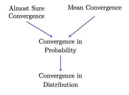
In this figure, the stronger types of convergence are on top and, as we move to the bottom, the convergence becomes weaker.

Convergence in Distribution

$$\lim _{n \rightarrow \infty} F_{X_{n}}(x)=F_{X}(x)$$

Also

$$\lim _{n \rightarrow \infty} p_{X_{n}}(x)=p_{X}(x)$$

Central Limit Theorem

Let $Z_{1}, Z_{2}, \cdots$ be a sequence of random variables having distribution functions $F_{Z_{n}}$ and moment generating functions $M_{Z_{n}}, n \geq 1$ , and let $Z$ be a random variable having distribution function $F_{Z}$ and moment generating function $M_{Z}$. If $M_{Z_{n}}(t) \rightarrow M_{Z}(t) $ for all $t$, then $F_{Z_{n}}(t) \rightarrow F_{Z}(t)$ for all $t$ at which $F_{Z}(t) $ is continuous.

$$P\left(\frac{X_{1}+\cdots+X_{n}-n \mu}{\sigma \sqrt{n}} \leq a\right)=P\left(\frac{\bar{X}-\mu}{\sigma / \sqrt{n}} \leq a\right) \rightarrow \frac{1}{\sqrt{2 \pi}} \int_{-\infty}^{a} e^{-\frac{x^{2}}{2}} d x \text { as } n \rightarrow \infty$$

Convergence in Probability

$$\lim _{n \rightarrow \infty} P\left(\left|X_{n}-X\right| \geq \varepsilon\right)=0 \text {, for all } \varepsilon>0$$

Markov’s inequality

$$P(X \geq a) \leq \frac{E[X]}{a}$$

Proof

For $a>0$ , define an event $A=\{X \geq a\}$ and $I_{A}$ an indicator for $A$ , that is

$$I_{A}=\left\{\begin{array}{ll}1 & \text { if } A \text { occurs }(X \geq a) \\ 0 & \text { if } A^{c} \text { occurs }(X<a)\end{array}\right.$$

Note that, since $X \geq 0, I_{A} \leq \frac{X}{a}$ and taking expectations of the preceding inequality yields

$$P(X \geq a)=P(A)=E\left[I_{A}\right] \leq \frac{E[X]}{a}$$

Chebyshev’s inequality

$$P(|X-\mu| \geq k) \leq \frac{\sigma^{2}}{k^{2}}$$

Weak Law of Large Numbers

$$\lim _{n \rightarrow \infty} P(|\bar{X}-\mu| \geq \varepsilon)\leq \frac{\sigma^{2}}{n\varepsilon^{2}}=0$$

Convergence in the r-th Mean

$$\lim _{n \rightarrow \infty} E\left(\left|X_{n}-X\right|^{r}\right)=0$$

Almost Sure Convergence

$$P\left(\omega \in \Omega: \lim _{n \rightarrow \infty} X_{n}(\omega)=X(\omega)\right)=1$$

Also

$$\mathbb{P}\left(\lim \sup \left\{\left|X_{n}-X\right|>\varepsilon\right\}\right)=0$$

由 Borel-Cantelli 推出

$$\sum_{n=1}^{\infty} P\left(\left|X_{n}-X\right| \geq \varepsilon\right)<\infty$$

Special distributions

Discrete random variables

1. Bernoulli $(p)$

   Description: $X$ indicates whether a trial that results in a success with probability $p$ is a success or not.

   Probability mass function: $p_{X}(k)=P(X=k)=\left\{\begin{array}{cc}p & \text { for } k=1 \ 1-p & \text { for } k=0 \ 0 & \text { otherwise }\end{array}\right.$

   Mean: $E[X]=p$

   Variance: $\operatorname{Var}[X]=p(1-p)$

   Moment generating function: $M_{X}(t)=1-p+p e^{t}$

2. Binomial$(n, p)$

   Description: $X$ represents the number of successes in $n$ independent trials when each trial is a success with probability $p$.

   Probability mass function: $p_{X}(k)=P(X=k)=\left\{\begin{array}{cc}\left(\begin{array}{l}n \ k\end{array}\right) p^{k}(1-p)^{n-k} & \text { for } k=0,1, \cdots, n \ 0 & \text { otherwise }\end{array}\right.$

   Mean: $E[X]=n p$

   Variance: $\operatorname{Var}[X]=n p(1-p)$

   Moment generating function: $M_{X}(t)=\left(1-p+p e^{t}\right)^{n}$

   Properties:

   • Binomial$(1, p)$=Binomial$(p)$

   • Sum of $n$ independent Binomial$(p)$ random variables is Binomial$(n, p)$

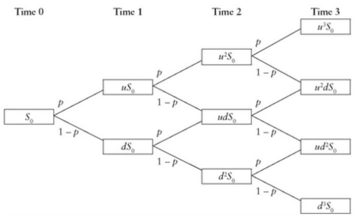
   • For Binomial tree model : $E[S_n]=S_0(pu+(1-p)d)^n$，$E[S_n^2]=S_0^2(pu^2+(1-p)d^2)^n$

     

1. Geometric $(p)$

   Description: $X$ is the number of trials needed to obtain a success when each trial is independently a success with probability $p$.

   Probability mass function: $p_{X}(k)=P(X=k)=\left\{\begin{array}{cc}p(1-p)^{k-1} & \text { for } k=1,2, \cdots \ 0 & \text { otherwise }\end{array}\right.$

   Cumulative distribution function: $P(X>n)=(1-p)^n$

   Mean: $E[X]=\frac{1}{p}$

   Variance: $\operatorname{Var}[X]=\frac{1-p}{p^{2}}$

   Moment generating function: $M_{X}(t)=\frac{p e^{t}}{1-(1-p) e^{t}}$

   Properties:

   • Geometric distribution is memoryless. That means that if you intend to repeat an experiment until the first success, then, given that the first success has not yet occurred, the conditional probability distribution of the number of additional trials does not depend on how many failures have been observed.
   • Discrete analogue of Exponential random variable.

2. Negative Binomial $(r, p)$

   Description: $X$ is the number of trials needed to obtain a total of $r$ successes when each trial is independently a success with probability $p$.

   Probability mass function: $p_{X}(k)=P(X=k)=\left\{\begin{array}{cc}\left(\begin{array}{c}k-1 \ r-1\end{array}\right) p^{r}(1-p)^{k-r} & \text { for } k=r, r+1, \cdots \ 0 & \text { otherwise }\end{array}\right.$

   Mean: $E[X]=\frac{r}{p}$

   Variance: $\operatorname{Var}[X]=r \frac{1-p}{p^{2}}$

   Moment generating function: $M_{X}(t)=\left(\frac{p e^{t}}{1-(1-p) e^{t}}\right)^{r}$

   Properties:

   • Negative Binomial$(1, p)$=Geometric$(p)$
   • Sum of $r$ independent Geometric $(p)$ random variables is Negative Binomial$(r, p)$
   • Discrete analogue of Gamma random variable
   • $P(X>n)=P(Y<r)$ for $Y$ a binomial random variable with parameters $n$ and $p$.

3. Poisson$(\lambda)$

   Description: $X$ is used to model the number of events that occur in many trials that has a small probability of occurrence.

   Probability mass function: $p_{X}(k)=P(X=k)=\left\{\begin{array}{cc}e^{-\lambda} \frac{\lambda^{k}}{k !} & \text { for } k=0,1, \cdots \ 0 & \text { otherwise }\end{array}\right.$

   Mean: $E[X]=\lambda$

   Variance: $\operatorname{Var}[X]=\lambda$

   Moment generating function: $M_{X}(t)=e^{\lambda\left(e^{t}-1\right)}$

   Properties:

   • A Poisson random variable $X$ with parameter $\lambda=n p$ provides a good approximation to a Poisson$(n, p)$ random variable when $n$ is large and $p$ is small.
   • If events are occurring one at a time in a random manner for which (a) the number of events that occur in disjoint time intervals is independent and (b) the probability of an event occurring in any small time interval is approximately $\lambda$ times the length of the interval, then the number of events in an interval of length $t$ will be a Poisson $(\lambda t)$ random variable.

4. Hypergeometric $(n, N, m)$

   Description: $X$ is the number of white balls in a random sample of $n$ balls chosen without replacement from an urn of $N$ balls of which $m$ are white.

   Probability mass function: $p_{X}(k)=P(X=k)=\left\{\begin{array}{cc}\frac{\left(\begin{array}{c}m \ k\end{array}\right)\left(\begin{array}{c}N-m \ n-k\end{array}\right)}{\left(\begin{array}{c}N \ n\end{array}\right)} & \text { for } k=0,1, \cdots \ 0 & \text { otherwise }\end{array}\right.$

   The preceding uses the convention that $\left(\begin{array}{l}r \ j\end{array}\right)=0$ if either $j<0$ or $j>r$.

   Mean: $E[X]=n \frac{m}{N}$

   Variance: $\operatorname{Var}[X]=n \frac{m}{N}\left(1-\frac{m}{N}\right)\left(\frac{N-n}{N-1}\right)$

   Property:

   • If each ball were replaced before the next selection, then $X$ would be a Binomial$(n, p)$ random variable.

Continuous random variables

1. Uniform $(a, b)$

   Description: $X$ is equally likely to be near each value in the interval $(a, b)$.

   Probability density function: $f_{X}(x)=\left\{\begin{array}{cl}\frac{1}{b-a} & a<x<b \ 0 & \text { otherwise }\end{array}\right.$

   Mean: $E[X]=\frac{a+b}{2}$

   Variance: $\operatorname{Var}[X]=\frac{(b-a)^{2}}{12}$

   Moment generating function: $M_{X}(t)=\left\{\begin{array}{cc}\frac{e^{b t}-e^{a t}}{t(b-a)} & t \neq 0 \ 1 & t=0\end{array}\right.$

2. Exponential $(\lambda)$

   Description: $X$ is the waiting time until an event occurs when events are always occurring at a rate $\lambda>0$.

   Probability density function: $f_{X}(x)=\left\{\begin{array}{cc}\lambda e^{-\lambda x} & x\ge0 \ 0 & \text { otherwise }\end{array}\right.$

   Cumulative density function: $F_X(x)=\left\{\begin{array}{cc}1-e^{-\lambda x} & x\ge0 \ 0 & \text { otherwise }\end{array}\right.$

   Mean: $E[X]=\frac{1}{\lambda}$

   Variance: $\operatorname{Var}[X]=\frac{1}{\lambda^{2}}$

   Moment generating function: $M_{X}(t)=\frac{\lambda}{\lambda-t}$ for $\lambda>t$

   Properties:

   • $X$ is memoryless, in that the remaining life of an item whose life distribution is Exponential $(\lambda)$ is also Exponential $(\lambda)$, no matter what the current age of the item is.
   • Continuous analogue of Geometric random variable.

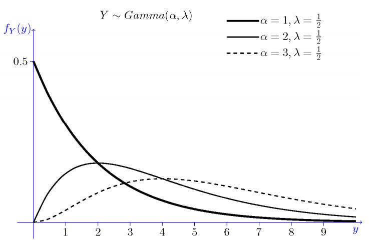
3. Gamma$(\alpha, \lambda)$

   Description: When $\alpha=n, X$ is the waiting time until $n$ events occur when events are always occurring at a rate $\lambda>0$.

   Probability density function: $f_{X}(x)=\left\{\begin{array}{cc}\frac{\lambda e^{-\lambda x}(\lambda x)^{\alpha-1}}{\Gamma(\alpha)} & x>0 \ 0 & \text { otherwise }\end{array}\right.$ where $\Gamma(\alpha)=\int_{0}^{\infty} e^{-x} x^{\alpha-1} d x$ is called the Gamma function.

   Using integration by parts, $\Gamma(\alpha)=(\alpha-1)\Gamma(\alpha-1), \Gamma(n)=(n-1)!$

   Mean: $E[X]=\frac{\alpha}{\lambda}$

   Variance: $\operatorname{Var}[X]=\frac{\alpha}{\lambda^{2}}$

   Moment generating function: $M_{X}(t)=\left(\frac{\lambda}{\lambda-t}\right)^{\alpha}$ for $\lambda>t$

   Properties:

   • Gamma$(1, \lambda)$=Gamma$(\lambda)$
   • If the random variables are independent, then the sum of a Gamma$\left(\alpha_{1}, \lambda\right)$ and a Gamma $\left(\alpha_{2}, \lambda\right)$ is a Gamma$\left(\alpha_{1}+\alpha_{2}, \lambda\right)$
   • The sum of $n$ independent and identically distributed exponentials with parameter $\lambda$ is a Gamma$(n, \lambda)$
   • $P\left(S_{n} \leq t\right)=P(N(t) \geq n)$, where $S_{n}$ has Gamma distribution with parameter $(n, \lambda)$ and $N(t)$ is Po isson with mean $\lambda t$.

   

4. Normal$\left(\mu, \sigma^{2}\right)$

   Description: In many real applications, a certain random variable of interest is a sum of a large number of independent random variables. We are often able to use the Central Limit Theorem to justify using the normal distribution.

   Probability density function: $f_{X}(x)=\frac{1}{\sqrt{2 \pi} \sigma} e^{-\frac{(x-\mu)^{2}}{2 \sigma^{2}}}$

   Mean: $E[X]=\mu$

   Variance: $\operatorname{Var}[X]=\sigma^{2}$

   Moment generating function: $M_{X}(t)=e^{\mu+\frac{1}{2} \sigma^{2} r^{2}}$

   Properties:

   • When $\mu=0, \sigma=1, X$ is called a standard nomal. If $X$ is Normal$\left(\mu, \sigma^{2}\right), Z=\frac{X-\mu}{\sigma}$ is standard normal.
   • Sum of independent normal random variables is also normal.
   • An important result is the Central Limit Theorem, which states that the distribution of the sum of $n$ independent and identically distributed random variables becomes normal as $n$ goes to infinity, for any distribution of these random variables that has a finite mean and variance.
   • Zero covariance of 2 nomal random variables implies these 2 variables are independent.

5. Lognormal$\left(\mu, \sigma^{2}\right)$

   Description: Lognormal random variable is often used as the distribution of the ratio of the price of security at the end of one day to its price at the end of the prior day.

   Probability density function: $f_{X}(x)=\left\{\begin{array}{cl}\frac{1}{x \sigma \sqrt{2 \pi}} e^{-\frac{(\ln x-\mu)^{2}}{2 \sigma^{2}}} & \text { if } x>0 \ 0 & \text { otherwise }\end{array}\right.$

   Mean: $E[X]=e^{\mu+\frac{1}{2} \sigma^{2}}$

   Variance: $\operatorname{Var}[X]=e^{2 \mu+\sigma^{2}}\left(e^{\sigma^{2}}-1\right)$

   Median: $x_{0.5}=e^{\mu}$

   Properties: $X$ is a lognormal random variable with parameters $\left(\mu, \sigma^{2}\right)$ if $Y=\ln X$ is a normal random variable with parameters $\left(\mu, \sigma^{2}\right)$, that is, lognormal $\rightarrow X=e^{Y \leftarrow \text { mamal }}$

6. Beta$(a, b)$

   Description: The $i$-th smallest of $n$ independent uniform $(0,1)$ random variables is a Beta$(i, n-i+1)$ random variable.

   Probability density function: $f_{X}(x)=\left\{\begin{array}{cl}\frac{\Gamma(a+b)}{\Gamma(a) \Gamma(b)} x^{a-1}(1-x)^{b-1} & 0<x<1 \ 0 & \text { otherwise }\end{array}\right.$ where $\Gamma$ is Gamma function.

   Mean: $E[X]=\frac{a}{a+b}$

   Variance: $\operatorname{Var}[Y]=\frac{a b}{(a+b)^{2}(a+b+1)}$

   Properties: Beta$(1,1)$ and Uniform $(0,1)$ are identical.